Detecting Low-Velocity Impact Damage in Composite Plates via a Minimization of Measured and Simulated Origin Approach
Gilad G1*, Brook A2, Uri Sol3
1 Department of Computer Science, University of Haifa, Israel.
2 Remote Sensing Laboratory, Center for Spatial Analysis Research (UHCSISR), Department of Geography and Environmental Studies, University of
Haifa, Mount Carmel, Israel.
3 NDT/E Laboratory, Israel Aircraft Industry (IAI), Israel.
*Corresponding Author
Gil Gilad,
Department of Computer Science, University of Haifa, Israel.
E-mail: giladgil@gmail.com
Received: June 20, 2016; Accepted: July 23, 2016; Published: August 03, 2016
Citation: Gilad G, Brook A, Uri Sol (2016) Detecting Low-Velocity Impact Damage in Composite Plates via a Minimization of Measured and Simulated Origin Approach. Int J Aeronautics Aerospace Res, S2:001, 1-13. doi: http://dx.doi.org/10.19070/2470-4415-SI02001
Copyright: Gilad G© 2016. This is an open-access article distributed under the terms of the Creative Commons Attribution License, which permits unrestricted use, distribution and reproduction in any medium, provided the original author and source are credited.
Abstract
In this paper, a new method for identifying impact locations applying a comparative simulated approach of minimization of measurement error against simulated data in a composite carbon plate-like structure using acoustic Lamb wave is proposed and reviewed. The purposed model detects impact locations by using an error minimizing algorithm based on the measured Lamb waves from an actual real impact and demonstrates a high-level of flexibility. Furthermore, the proposed model can be straightforwardly calibrated for different velocities and other parameters inherent in carbon-based structures, reducing the effects of the structure’s anisotropic properties. In particular, the time of arrival of an impact signal is calculated by applying wavelet transform and threshold crossing methods. Experiment results illustrate the effectiveness of the proposed method by presenting a very accurate detection rate of real low-velocity impacts on a carbon-based plate-like structure. This promising technique enables inspection and on-line monitoring of impacts on composite structures. Further developments of the suggested model are discussed, and are mainly focused on producing a velocity independent extension mode.
2.Introduction
3. Methodology
3.1. Lamb waves
3.2. TOA Determination
3.3 Impact detection
4. Results
4.1. Experimental setup and velocity test
4.2. Experimental results
5.Discussion
6.Conclusion
7.Acknowledgements
8.References
Keywords
Wavelet; Acoustic Emission; Impact location; Lamb Wave; Non-Destructive Testing.
Introduction
The increasing usage of carbon-based composite in aeronautic and aerospace industries introduces new demands and raises new challenges on real-time monitoring modes and demands for highlevel accuracy, non-detractive testing, and evaluation (NDT/E). These materials are recognized for their high toughness, mechanical resistance, immunity to corrosion (metallic components) and their very light weight [1].
In most of the cases, the low energy of an impact will not indent the surface, yet it will reduce the loading resistance and decrease the integrity of layer adhesion. In some rare cases, some visible cracks might appear. Thus, the main detection and evaluation of damages in composites are guided by the fact that damages and defects are not visible or visually recognizable and might occur in many different forms. Yet, these damages and defects could reduce the overall strength of the composite component. Facing these problems, different NDT/E and non-contact methods and techniques suitable for impact damages and defects are much needed. Up to now, methods such as infrared thermography [2], X-Ray Radiography [3], ultrasonic inspection [4], mechanical independent analysis, and 3-D computed tomography [5] are used to evaluate the defects on specimens. Recently, the Lamb waves, or elastic ultrasonic waves, which exist in thin plate-like structures, are successfully implemented by structural health monitoring (SHM) systems. Due to a low material and geometrical attenuation and respectively narrow wavelength, Lamb waves interact even with low levels of damage [6]. However, the complex properties concerning existence of at least two basic modes, a symmetric (S0), and simultaneously, an anti-symmetric (A0) mode, which under special conditions can convert into each other (particularly in composite materials) must be addressed and reduced before the data can be utilized for signal processing and information extraction. Nevertheless, the Lamb waves are interesting for monitoring of light-weight CFRP (carbon fiber reinforced plastics) structures,and for real-time monitoring purposes. Unlike other approaches that detect structure damage after it has evolved, by using Lamb waves, real-time damage interpolation can be detected.
While numerous solutions previously proposed for aluminum structures, the anisotropic nature of composite materials makes the problem even more complex. The ability to locate an acoustic emission (AE) source for monitoring structural integrity might reveal the formation of cracks and impacts. The majority of methods are based on the time of arrival (TOA) of the AE signal using a triangulation technique in order to estimate the location of an AE; e.g., an impact. In carbon-based material, where the velocity may differ in relation to the angle on which the AE signal propagates, such approach may cause a significantly large error, since any noise can drastically alter the result. In deterministic triangulation-based methods, the TOA is mainly evaluated by threshold-crossing peak-signal correlation [7], and recently, the continuous-wavelet-transform (CWT) has been engaged for that purpose. The most recent studies proposed the CWT as a method of finding the TOA of dispersive AE waves [8-11]. All these methods are based on prior knowledge by requesting the sensor location and velocity of the AE signal before estimating the impact location, mainly using triangulation technique [12-14,15]. As previously mentioned, these methods can be considered as deterministic methods and since the velocity of the AE wave is strongly dependent upon orientation, they underperformed on composite materials.
The alternative approach utilizes a probabilistic principle in order to estimate the location of an AE source [10]. The main assumption of these models is that due to the physical properties of the material and physical principles of the deterministic approaches both error and uncertainties are always unavoidable, even when using the CWT method. Therefore, these methods must yield an internal (inherent) error. However, even though these methods do allow for an uncertainty in the wave velocity, they do not account for the orientation-dependent property of a composite structure [11].
In fact, the majority of studies combine parts of the probabilistic approaches with the orientation-dependent wave velocity of the composite in order to improve the AE source location in a platelike structure [16-19]. Numerous studies are developing a simulated procedure in order to incorporate noise level and identify the AE source location. These experimental studies are conducted on several composite panels in order to validate and further develop the suggested algorithm.
The main aim of the present study is to apply a simulating approach in order to estimate the AE location on carbon-based plate-like structures, with a durable noise-reduction technique and a velocity independent model. Experimental study of dedicated stiffened carbon-epoxy panels is being conducted to validate the proposed localization method.
Methodology
Lamb-wave theory refers to the movement of mechanical waves in a thin free plate. The waves move on the upper and lower parts of the free plate. This theory is developed and documented in a multiple number of textbooks and articles [14, 16]. The following section will introduce the basic concept for the analysis of such waves.
The wave equations are presented by Equations 1 and 2.
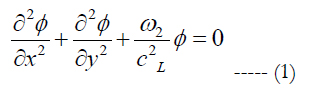
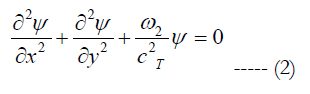
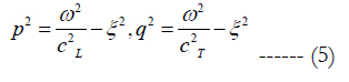
Where Φ and Ψ are two potential functions,c²L = (λ + 2µ ) / ρ and c²T = µ / ρ are the pressure and shear wavespeeds, λ and µ are the Lame constants, and ρ is the density. It is assumed that the time dependence is harmonic in the form of e-iωt. Therefore, the solution of Equation 1 is given by Equations 3, 4 and 5.
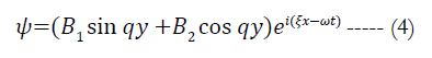
Where ξ = ω / c is the wave number and
The four integration A1,A2,B1,B2 constants will be found by the boundary conditions. Using the relations between them result in Equations 6 and 7.
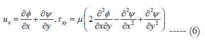
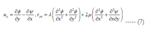
From that we obtain


There exist two forms of motion, symmetric and anti-symmetric, which correspond to the two Equations 9 and 10. In order to calculate free wave motion, the homogenous solution needs to be derived by applying the stress-free boundary condition at the surfaces (y = ± d where d is half the thickness of the plate) so that the compact form known as the Rayleigh-Lamb equation can be obtained:
Where +1 describes the symmetric (S) mode and -1 describes the anti-symmetric mode (A).
There is an inherent relationship between these equations, in particular the angular frequency ω and the wave number along with other coefficients that yield different Lamb-mode shapes designated as:
Single Reference Frame
A good example for a steady-state single rotating flow region problem is the Couette flow (see Figure 1), where the entire flow regime is confined between two rotating cylinders. The twodimensional Couette flow is steady, but it develops the Taylor instability for increasing Taylor number.
S0,S1,S2,.... and A0,A1,A2.....
Corresponding to symmetric and anti-symmetric respectively. Due to this relationship, the wave speed will change according to the excitation frequency and produces wave dispersion. For every plate thickness and frequency, the predicted wave speed will change. This model is for isotropic infinite plates. While in reality the carbon-based composite are neither isotropic nor infinite. This model gives a close approximation and understanding for the behavior and interaction of waves in a plate and with delamination. By using TOA analysis of Lamb waves, the impact location can be predicted and estimated.
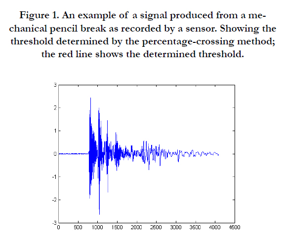
Figure 1. An example of a signal produced from a mechanical pencil break as recorded by a sensor. Showing the threshold determined by the percentage-crossing method; the red line shows the determined threshold.
A superposition of longitudinal and shear modes are the fundamental parameters of guided Lamb waves. The propagation characteristics of these waves vary with entry angle, excitation, and structural geometry. A Lamb mode can be either symmetric (S0) or anti-symmetric (A0) as formulated by [20]. Detailed experimentally measured attenuation coefficients of Lamb waves in different composite structures are reported by [21].
For a given material, the Lamb-wave frequency is related to the wave number and plate geometry. The dispersion of an AE source mainly corresponds to the dispersive curves of infinite Lamb modes. While both modes are excited directly by the source, after some time the modes are clearly separated. This phenomenon is explained by the different wave velocities, whereas the reflected or converted modes are named in a different manner. If a Lamb wave is excited by an impact event, at least two primary groups of waves travel through the plate with different propagation velocities. Such as, the group velocity of the A0-mode varies for the different frequencies it is excited with different group velocities. In this study, several different methods for extracting the TOA from an AE event signal are examined.
A threshold of 25 dB is defined as the TOA of the AE signal. This value was determined based on the average environment noise. In several experiments, a smaller negative value is defined as a threshold, this negative value is supported by an observation that white noise values rarely crosses the zero value while actual impact signal normally crosses it. This method works relatively well for small distances of wave propagation. However, since AE signals are dispersive, these methods might be influenced by attenuation that causes a lag in time determination in relation to the distance, since sensors that are positioned further from the AE location will have a lower maximum amplitude and a fixed threshold will be triggered by different points of the wave. In order to overcome this lag, a percentagebased threshold-crossing method was introduced. The threshold is determent by a certain percentage of the signal’s peak value (Equation 12).
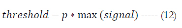
Where p is the percentage of the signal and max (signal) is the peak value of the signal as illustrated in Figure 1 on a recorded pencil-break signal.
The CWT is employed on the recorded AE signal in order to convert it to a time-frequency domain used to extract the time. This method is executed by the following modes: first, a mean of all wavelet scale-intensities is calculated, resulting in a time mean-intensity plot. On this plot, a threshold is used to determine the TOA. The second mode applies a specific scale of the wavelet map calculated with the Moral function. Usually a scale of ten is used corresponding to the S0 mode, although one can use a scale with maximum correspondences with other propagating modes optimized to the recorded AE signal. On the intensity plot of the specific scale, the TOA is determent by a threshold.
The applied CWT is described by Equation 13, where a > 0 and * denotes a complex conjunction, a is the scale of the function in the WT that corresponds to the frequency; and b is a shift variable of the function, which is a shifting and scaling variables of the original wavelet ψ(t).
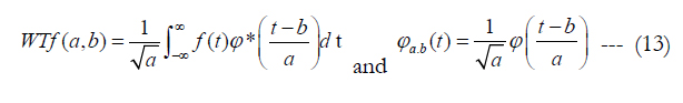
In WT, there is a relation between the scale factors 'a' to the signal frequency; higher scales correlate with a higher frequency. One can view the process as a sliding window for both parameters a and b, where changing a yields a different frequency correlation and changing b yields the correlation of the function of a specific part of the input function (signal) ƒ(t).
In this study, the Morlet function is used as the wavelet mother function. The Moral function satisfied the mother function conditions and is defined by Equation 14.
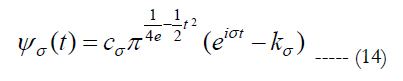
Where kσ = e-1/2σ2 is defined by the admissibility criterion and the normalization constant cσ (Equation 15).
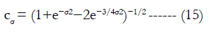
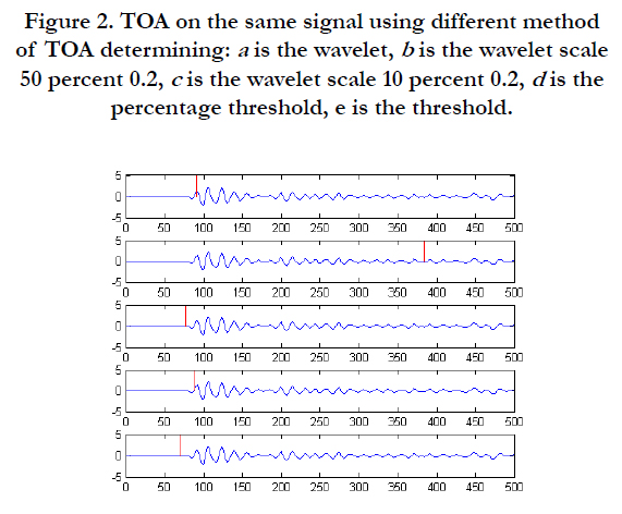
Figure 2. TOA on the same signal using different method of TOA determining: a is the wavelet, b is the wavelet scale 50 percent 0.2, c is the wavelet scale 10 percent 0.2, d is the percentage threshold, e is the threshold.
In order to identify the impact location, the proposed model utilizes a minimization technique, for minimizing the error between a measurement of AE TOA and a simulated TOA from a specific location. For an AE caused by an impact, the TOA is determined based on the methods in Section 2.1. The AE signal is detected by PZT sensors, whereas the AE event is defined to be a signal that is stronger than a threshold of 25 dB in all sensors. Once an AE event is detected, the TOA is extracted from the detected signals and each sensor is stamped with a time relative to a global experiment time. Once obtained the measured time is then considered to be a true AE event time. Between each sensor pair si,sj, the time delta (differences) is calculated and is defined to be the measured delta time of arrival and noted as ΔtijM. An AE event is then simulated by assuming that a wave has started to propagate from a point (x impact,y impact) at a certain velocity V that may vary depending on its orientation relative to the panel and then calculating the TOA to each of the sensors based on their known position.
For real carbon-based plate-like structures with N sensors, a threshold is set above the background noise to initialize the recording of the signal by the sensors. Once the signal crosses the threshold, it is recorded and viewed as an AE event. The initial time of the AE is unknown; therefore, the time differences between the sensors are calculated. Recording sensors have an internal global time that is used for synchronization purposes between sensors, from TOA relative to the global experiment time. The time differences are derived according to Equation 16.
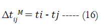
Where ti,tj are TOA determined from the signal based on the method in Section 2.1 relative to the global experiment time, where ΔtijM is the measured time difference between a sensor pair i, j. Note that for N sensors there are N(N-1)/2 sensors pairs; the multiplicity in the number of sensors is beneficial for both measurement TOA noise reduction and error- cancelation in velocity estimation. In the proposed model, the AE wave propagation velocity in a composite and its resulting delta TOA is defined by Equation 17.
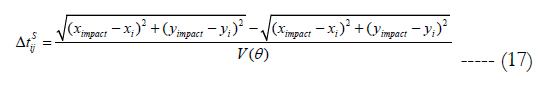
Where (x impact,y impact) are the coordinates of the simulated impact and (xj,yj) are the ith and jth sensor coordinates, v(θ) is the AE wave velocity in direction θ, at a specific frequency. In the presented study, the velocity is treated as a constant in every direction of panel orientation; i.e., ∀ θ: v(θ) = constant, although in real life this is not necessarily the case. In this study, it yielded sufficient results. However, the suggested model can take into account and simulate the change in velocity in relation to panel orientation if the velocity to orientation dependency function is known. In order to find the most likely AE event source location, an intensive search for (x impact,y impact) coordinates minimized the following expression (Equation 18).
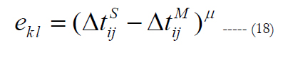
Where eij is a matrix, cell k, l holds the difference between the simulated delta TOA and the measured delta TOA for a sensor pair i, j. This can be viewed as a map where each point on the map shows the similarity between the measured delta TOA and the simulated delta TOA for that point on the map. Cells k, l correlate to a location on the panel with coordinates of (x impact,y impact) depending on the simulating grid density and range, and µ is a tolerance parameter used to adjust the error generality. Small values (<1/2) yield a more specific location by giving small-error values only for the points on the map with very low differences. Large values (>2) yield a broader estimation of location in the map by allowing for not so small differences to have a small value as illustrated in Figure 5.
In Equation 19, E is the sum of all the error “maps” between each sensor pair. We will choose x impact,y impact) that minimizes the combined error maps as the predicted point of AE event source location.
According to Figure 4, if a wave’s propagating velocity is constant and does not change in respect to panel orientation; two sensors can be viewed as defining a parabolic line for a constant time difference (parameter C). For a given time difference C between two sensors (e.g., CH1 and CH2), every point on the following parabolic line will generate a wave propagation that will result in the time difference C between the TOA to sensor CH1, CH2 as illustrated in Figure 4. By using more than two sensors, the parabolic lines created by each sensor pair will intersect at the point of impact or origin of the wave propagation.
In reality, due to the inherent uncertainty level of the measurement, the parabolic line only represents the lowest difference between the delta TOA of two sensors and the simulated AE event location delta TOA, namely "error map." Since the final AE event impact location estimation is the combination of all sensor pairs and their corresponding error maps, the value of µ (given in Equation 18) has a significantly strong effect on prediction and error cancelation: High values of µ make for a wider spread on the lowest error line; and a low value makes for a sharper lowest error line, as illustrated in Figure 5.
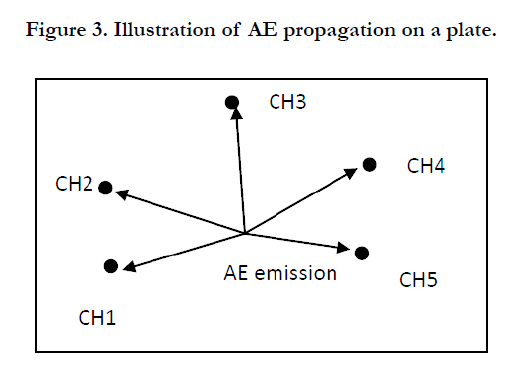
Figure 3. Illustration of AE propagation on a plate.
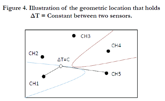
Figure 4. Illustration of the geometric location that holds ΔT = Constant between two sensors.
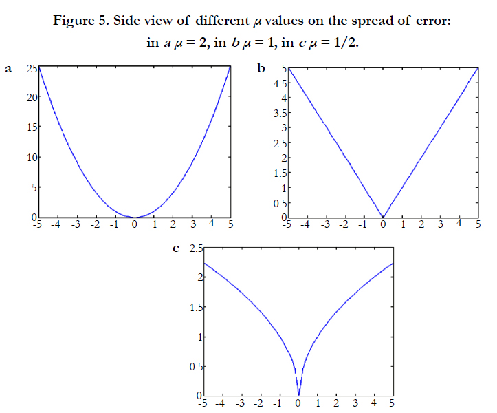
Figure 5. Side view of different μ values on the spread of error: in a μ = 2, in b μ = 1, in c μ = 1/2.
Results
A setup consists of two carbon-fiber woven fabric, epoxy preimpregnated reinforced polymer (CRFP) panels in various sizes, and an AEwin Mistras system (with 8-channel, 16 bit, 400 kHz bandwidth, PCI bus-card capable of simultaneously recording data from eight PZT sensors) is used to test the proposed model. The panel dimensions are 593 x 590 mm. Both have 12 layers of carbon fiber in an alternating 0/90-45/45 orientation. The system includes eight 180 kHz main-frequency 14 mm circular PZT sensors amplified by a 43 dB pre-amplifier. The sensors are denoted S1-S8, and are placed in various configuration on the CRFP panels. Both a full 8-sensor configuration and more moderate 5-sensor configuration are tested and recorded. Figures 6 and 7 illustrate the panel and sensor locations (Table 1), as well as known impact locations (Table 2). Using our method for identifying TOA we avoided the echo from boundary conditions, also we gave a small gap and reinforce the edges of the plates with dampers to lower their effects.
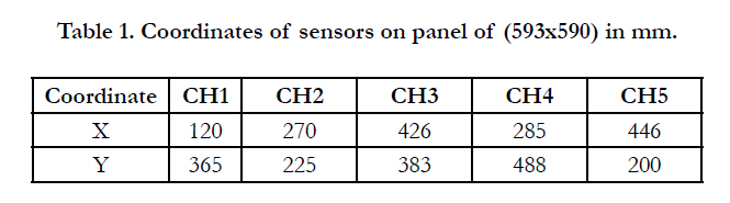

Table 1. Coordinates of sensors on panel of (593x590) in mm.
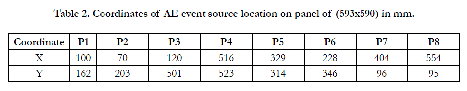
Table 2. Coordinates of AE event source location on panel of (593x590) in mm.
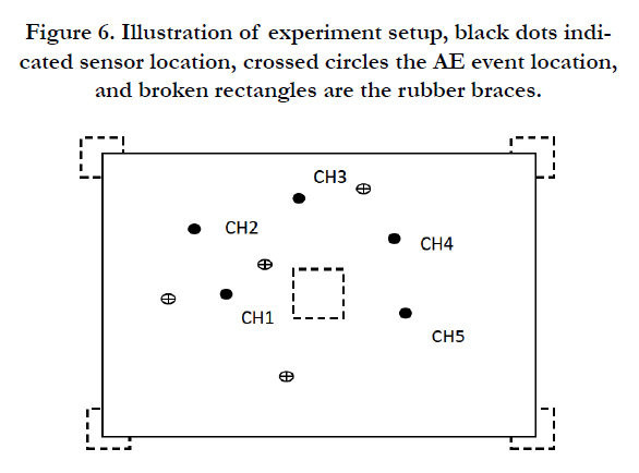
Figure 6. Illustration of experiment setup, black dots indicated sensor location, crossed circles the AE event location, and broken rectangles are the rubber braces.
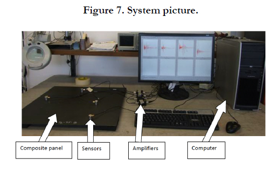
Figure 7. System picture.
In the present study, both mechanical pencil-lead break and steelball drop are used to induce the AE event, a single impact produced by the mechanical pencil as the tip break which allows for a more control measurement and separation of signal location. With the steel ball there are secondary impacts as the ball bounces following the first impact, to avoid referring to secondary impact signal only the first AE event from all sensors is captured and processed. For the location prediction, a fixed velocity is used, even though it is possible to decrease error by using the directiondependent velocity profile of the panels to simulate AE wave propagation velocity instead of a fixed velocity in every direction, which was not used in this study since the profile was unknown. Likewise, the model’s inherent degree of freedom allows estimating the AE event source location without any prior knowledge of group velocity. In fact, a suggested method is finding a velocity that minimizes the error area on the map or choosing a velocity that minimizes the uncertainty of impact location prediction characterized by a minimal error estimation value. This aspect of the study needs further research but initial result indicates that by choosing a specific velocity for every impact the estimation location error can decrease.
An additional experiment is conducted in order to confirm the previous results. In this experiment, an 8-PZT sensor setup is suggested. The sensors are placed on the panel in a grid formation (see detailed coordinates in Table 3 and Figure 8) and AE impact events from three different locations are induced using pencil-lead break.
The three impacts are located internally or inside the sensor field (see detailed coordinates in Table 4 and Figure 8). The estimated velocity of 5700 m/s is used as the model velocity.
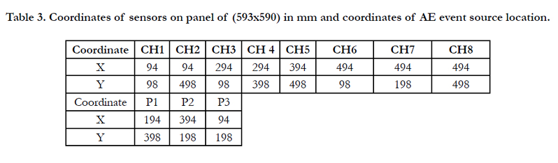
Table 3. Coordinates of sensors on panel of (593x590) in mm and coordinates of AE event source location.
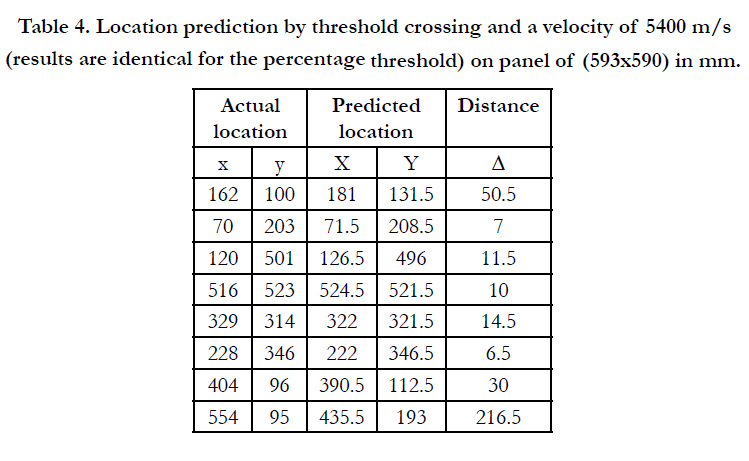
Table 4. Location prediction by threshold crossing and a velocity of 5400 m/s (results are identical for the percentage threshold) on panel of (593x590) in mm.
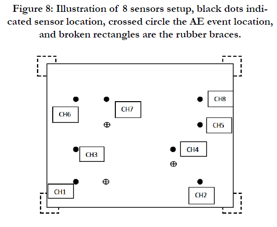
Figure 8: Illustration of 8 sensors setup, black dots indicated sensor location, crossed circle the AE event location, and broken rectangles are the rubber braces.
A velocity determining experiment is conducted to measure the AE group velocity. In this experiment, two sensors with a distance of 400 mm between them are placed on a 12-layered panel woven in a 0/90, -45/45 pattern of size 593 x 590 mm. The AE emission is induced on top of these two distanced sensors. The first sensor acts as a trigger and the TOA from sensor A to sensor B is measured. The experiment was repeated for different ranges of AE emission location starting at 50 mm to 150 mm ahead of sensor A. Furthermore, testing the influence of panel orientation on the velocity, the sensors rotated 10 degrees with respect to the panel boarders until completing 90 degree then repositioned in another corner as illustrated in Figure 6.1. The velocity is concluded to be around 5400 m/s with a variance of 500 m/s depending on the orientation angle.
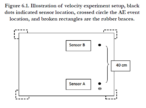
Figure 6.1. Illustration of velocity experiment setup, black dots indicated sensor location, crossed circle the AE event location, and broken rectangles are the rubber braces.
The modeled results for predicting the AE source location is presented in Figure 9, showing the different impacts and their corresponding predicted location. The numerical results are reported in Tables 4, 5 and 6.
Following the results of the velocity experiment, this model uses a fixed velocity of 5400 m/s. The TOA is obtained using all the previously described methods (sub-paragraph 2.1). Both µ values (µ= 2 in Table 4 and µ = ½ in Table 5) are used to predict the location by calculating the error estimator every 0.5 mm. Tables 10-11 show the prediction errors using various 𝜇 values. One can see that it produces slightly different results. The error maps are shown in Figure 10.
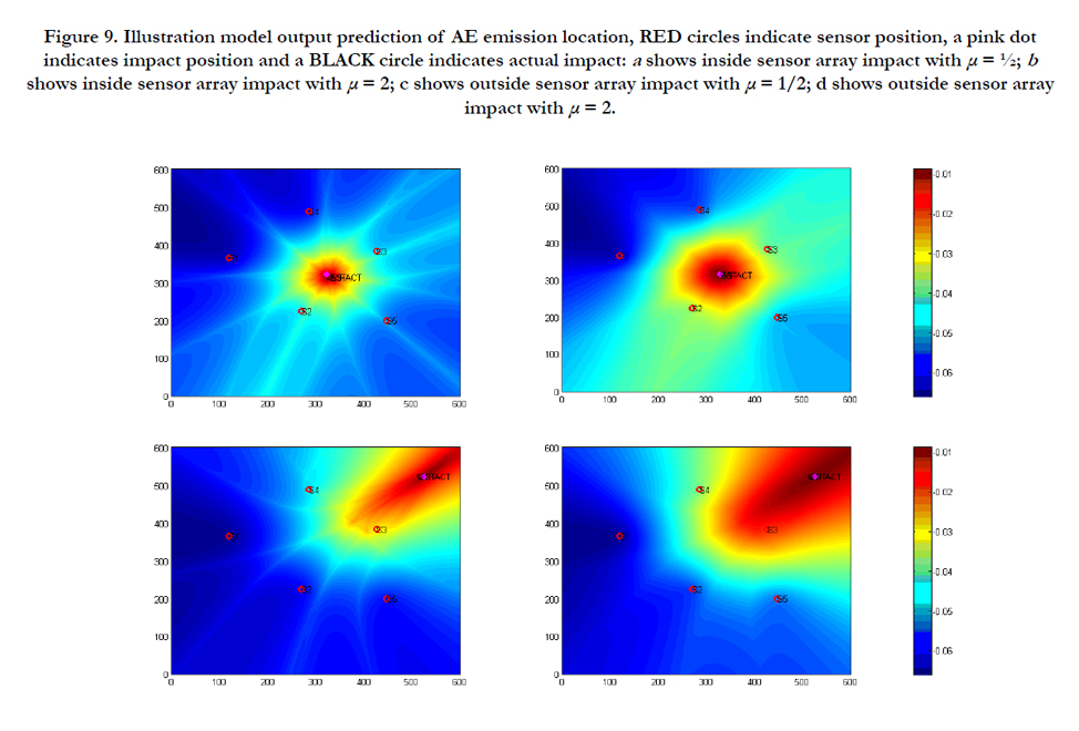
Figure 9. Illustration model output prediction of AE emission location, RED circles indicate sensor position, a pink dot indicates impact position and a BLACK circle indicates actual impact: a shows inside sensor array impact with μ = ½ b shows inside sensor array impact with μ = 2; c shows outside sensor array impact with μ = 1/2; d shows outside sensor array impact with μ = 2.
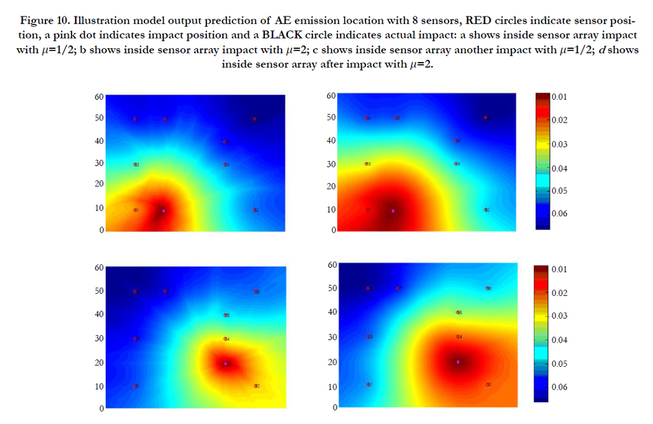
Figure 10. Illustration model output prediction of AE emission location with 8 sensors, RED circles indicate sensor position, a pink dot indicates impact position and a BLACK circle indicates actual impact: a shows inside sensor array impact with µ=1/2; b shows inside sensor array impact with µ=2; c shows inside sensor array another impact with µ=1/2; d shows inside sensor array after impact with µ=2.
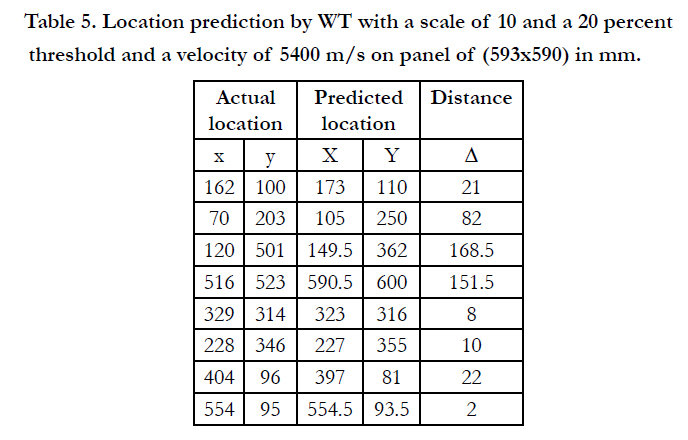
Table 5. Location prediction by WT with a scale of 10 and a 20 percent threshold and a velocity of 5400 m/s on panel of (593x590) in mm.
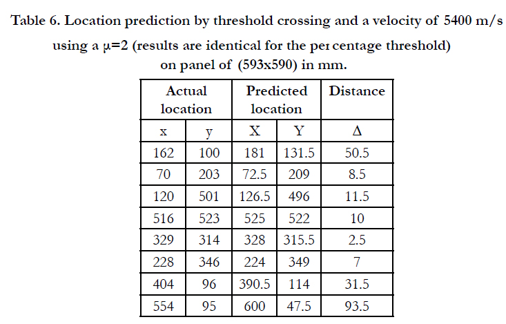
Table 6. Location prediction by threshold crossing and a velocity of 5400 m/s using a μ=2 (results are identical for the percentage threshold) on panel of (593x590) in mm.
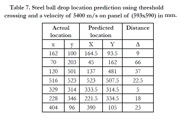
Table 7. Steel ball drop location prediction using threshold crossing and a velocity of 5400 m/s on panel of (593x590) in mm.
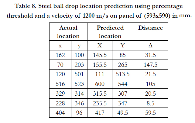
Table 8. Steel ball drop location prediction using percentage threshold and a velocity of 1200 m/s on panel of (593x590) in mm.
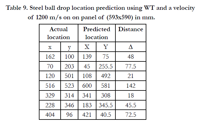
Table 9. Steel ball drop location prediction using WT and a velocity of 1200 m/s on on panel of (593x590) in mm.
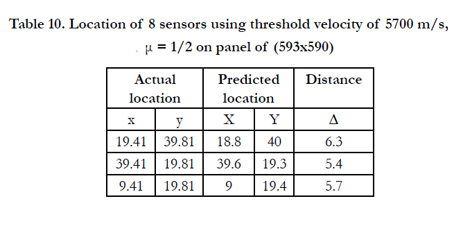
Table 10. Location of 8 sensors using threshold velocity of 5700 m/s, μ = 1/2 on panel of (593x590) in mm.
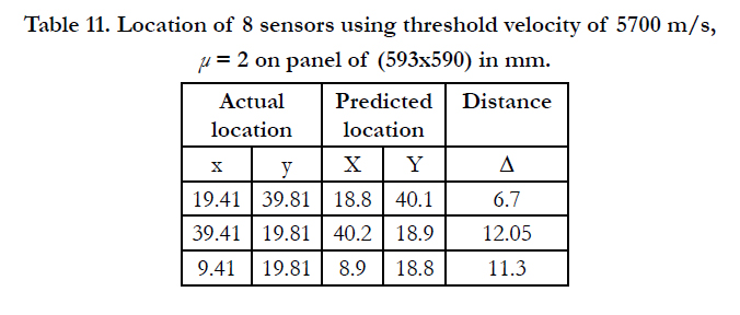
Table 11. Location of 8 sensors using threshold velocity of 5700 m/s, μ = 2 on panel of (593x590) in mm.
It is notable that the detection accuracy is highly correlated to the location of an impact or AE event source location. The prediction is more accurate for an interpolated location rather than an extrapolated location. This can be explained by the fact that inside the sensors field there will be a stabilizing effect by the opposite sensor that will in fact reduce error in location due to mistaken initial velocity estimation. Thus, each sensor will over/under estimate the location, and the two will reduce the overall error. Figure 11 shows a case where the input velocity was higher than the physical velocity. Since four sensors over predicted the location, the one sensor left did not have enough influence to stabilize the error resulting in a shifted location of the AE event the figure also illustrates the influence of sensor deployment on prediction location of an AE event.
However, in the extrapolation scene, when the impact is outside of the sensor field, the input velocity error will not have that stabilizing effect. In this case, since none of the sensors can stabilize the error, the velocity estimation inaccuracy has an effect on the location prediction and therefore, the estimated location can be closer or further than the actual one.
Nevertheless, this property can be used to calibrate the velocity of any unknown panel. One creates an impact outside the sensor field with a general estimation of the velocity and then change the velocity until the predicted location is matched with the actual impact. Certainly, in an anisotropic composite panel the velocity will be accurate only for that panel orientation. Yet, the presented study results show a relatively high-accuracy level, despite the lack of the true orientation/velocity dependence information. Furthermore, the proposed model can be auto-calibrated to a velocity by choosing an input velocity that minimizes the low-error area (Figures 12a, 12b, 12c) marked as the red area. Since the area of low error is determined by a parabolic line from a pair of sensors and their correlated TOA difference, if the area is small all sensors pairs agree internally and the input velocity for the predicted error is accurate.
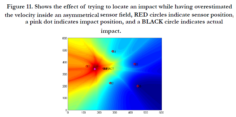
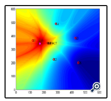
Figure 11. Shows the effect of trying to locate an impact while having overestimated the velocity inside an asymmetrical sensor field, RED circles indicate sensor position, a pink dot indicates impact position, and a BLACK circle indicates actual impact.
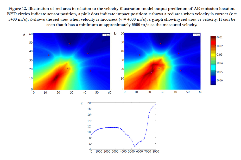
Figure 12. Illustration of red area in relation to the velocity-illustration model output prediction of AE emission location. RED circles indicate sensor position, a pink dots indicate impact position: a shows a red area when velocity is correct (v = 5400 m/s); b shows the red area when velocity is incorrect (v = 4000 m/s); c graph showing red area vs velocity. It can be seen that it has a minimum at approximately 5500 m/s as the measured velocity.
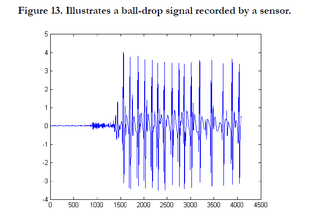
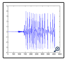
Figure 13. Illustrates a ball-drop signal recorded by a sensor.
Further study is required to confirm this assumption and accelerate the running time. In the present experiments, the area size/ velocity graph is not concave and the calculation of the minimum value is time consuming.
Ball-drop impact produces several wave modes and relatively different AE signal form in comparison to the pencil break, as shown in Figure 13. To account for the change, the TOA method parameters were slightly altered as indicated in Table 7-9. The different AE signal characteristics demand a different calibration mode.
The eight-sensor configuration was also examined. Its error map is shown in Figure 12. The multiplicity of sensors resulted in improved predictions as illustrated in Tables 10 and 11 with different µ values.
Theoretically this model is limited to 3 sensors as the minimal number of sensors that will yield usable results. Every addition of a sensor will provide a higher guarantee of the impact location up to a limit. As discussed the orientation of sensors and their collaboration in combining the data also plays a rule in the outcome of predicted location due to their ability to cancel each other error in the event of measurement of speed estimation error. Table 12 illustrate the behavior of the model with different number of sensors. To produce this table we simply excluded sensors from the computation of the model from sensor 8 – 3 regardless of its position on the board. Which yield interesting result, as seen in impact 2 in the table (P2) followed by several subtraction of sensor the prediction became an extrapolated problem rather than interpolated one resulting in a poor measurement cancelation ability and a large estimation problem.
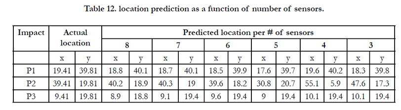
Table 12. location prediction as a function of number of sensors.
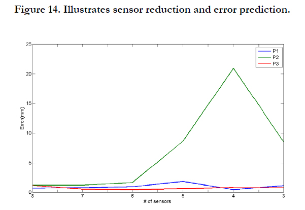
Figure 14. Illustrates sensor reduction and error prediction.
Discussion
In this paper, a novel approach for locating AE source emission on carbon-fiber material was presented. The model was developed and tested on real CFRP panels, emphasizing the presence of surrounding noises. As opposed to [15] there the CWT is applied to determine TOA using a deterministic triangulation approach or [10] that proposes a truly probabilistic approach; the suggested model combines both cases along with a basic concept proposed by [11] to create a flexible method for determining the AE source emission location. While [10] focused his work on aluminum plates, we conducted our testing on composites and enabled an orientation-dependent velocity approach that tackled the anisotropic nature of composite panels [11]. raised questions and pointed to the need for advanced methods for composite materials.
While [10] presented a solid probabilistic approach to locating AE emissions, his work was tested on aluminum plates with a unified orientation velocity pattern. This structure is uncommon in carbon-fiber plates due to its anisotropic nature. Therefore, a probabilistic approach may result with too many contradicting dimensions that overloaded the algorithms [15]. presented a triangulation approach, retrieving highly accurate results, while limiting the information to only three sensors. This combine data property helps in reducing both errors in measurement and in velocity [11]. Reported high-accuracy results applying both wavelet and a quadratic dividing scheme for assessing the AE source location. These approaches drove our model to investigate both wavelets as a TOA-finding technique and resulting in simulating finding the source location.
Conclusion
This paper presents an investigation of the ability to predict the location of an AE source for a carbon composite based platelike structure while considering the anisotropic properties of carbon-based materials and measurement uncertainties. TOA of the wave emission is determined using several approaches such as CWT and threshold-crossing. Once the true TOA were obtained, a simulating model was developed to predict the AE source location. The model is velocity dependent but can be calibrated easily in a real world application, and given the composite orientation dependency pattern, the velocity can be modified to predict with ever greater accuracy. The experimental study on carbon-fiber plates showed that the prediction is more robust inside the sensor field and unlike deterministic approaches; the presented model provided a likelihood of an AE source location and enabled autocalibration of the velocity.
Acknowledgements
The authors thank the NDT/E Laboratory at the Israel Aircraft Industry for funding this study and providing the required equipment for the presented experiments.
References
- Sheen DM, McMakin DL, Hall TE, Severtsen RH. (2009) “Active millimeter- wave standoff and portal imaging techniques for personnel screening,” in Proc. IEEE Conf. Technolo. Homeland Security, Boston, MA. 440–447.
- Salazar A, Vergara L, Llinares R. (2010) Learning Material Defect Patterns by Separating Mixtures of independent Component Analyzers from NDT Sonic Signals. Mechanical Systems and Signal Processing, 24(6): 1870-1886.
- Krumm M, Kasperl S, Franz M. (2008) Reducing non-linear artifacts of multi-material objects in industrial 3D computed tomography. NDT and E International. 41(4): 242-251.
- Cantwell WJ, Morton J. (1996) The impact resistance of composite materials: a review, Composite. 22(5): 347-362.
- Appleby R (2004) Passive millimetre-wave imaging and how it differs from terahertz imaging, The Royal Society 379- 394.
- Mook G, Pohl J, Michel F (2003) Non-destructive characterization of smart CFRP structures. Smart Mater. Struct. 12: 997-1004.
- Ziola SM, Gorman MR (1991) Source location in thin plates using crosscorrelation. Journal of the Acoustical Society of America. 90(5): 2551-2556.
- Jeong H, Jang YS. (2000) Wavelet analysis of plate wave propagation in composite laminates. Composite Structures. 49(4): 443-450.
- Hamstad MA, A O’Gallagher A, Gary J (2002) A wavelet transform applied to acoustic emission signals: part 1 source identification. Journal of Acoustic Emission. 20: 39-61.
- Tobias A. (1976) Acoustic emission source location in two dimensions by an array of three sensors, Non-Destructive Testing. 9(1): 9-12.
- Gaul L, Hurlebaus S. (1998) Identification of the impact location on a plate using wavelets. Mechanical System and Signal Processing. 12(6): 783-795.
- Salehian, Armaghan (2003) Identifying the location of a sudden damage in composite laminates using wavelet approach. Diss. Worcester Polytechnic Institute.
- Yan Gang, Jianfei Tang. (2013) A Bayesian approach for acoustic emission source location in plate-like structure. In procedure of SINCE2013, Singapore International NDT Conference & Exhibition, Singapore.
- Yamada H. (2000) Lamb wave source location of impact on anisotropic plates. Journal of Acoustic Emission 18: 51.
- Ciampa F, Meo M. (2010) Acoustic emission source localization and velocity determination of the fundamental mode A0 using wavelet analysis and a Newton-based optimization technique. Smart Materials and Structures.19(4): 045-027.
- Niri ED, Salamone S (2012) A probabilistic framework for acoustic emission source localization in plate-like structures. Smart Materials and Structures. 21(3): 035009.
- Beck JL, Katafygiotis LS (1998) Updating models and their uncertainties i:Bayesian statistical framework. ASCE Journal of Engineering Mechanics. 124(4): 455-461.
- Nichols JM, Link WA, Murphy KD. (2010) A Bayesian approach to identifying structural nonlinearity using free-decay response: application to damage detection in composites. Journal of Sound and Vibration. 329(15):2995-3007.
- Yan GA. (2013) A Bayesian approach for damage localization in plate-like structure using Lamb waves. Smart Materials and Structures. 22(3): 035012.
- Achenbach JD. (1973) Wave propagation in elastic solids, Amsterdam, North–Holland.
- Pierce S, Staszewski W, Gachagna A, James I, Philp W, et al. (1997) Ultrasonic Condition Monitoring of Composite Structures Using a Low Profile Acoustic Source and an Embedded Optical Fibre Sensor, SPIE conference Smart Structure & Materials. 3041: 3-6.