Experiences Plan Approach for Static Pressure Reliability; Case Study: Aircrafts Pitot Sensors
Ezzeddine W*, Schutz J, Rezg N
University of Lorraine, France.
*Corresponding Author
Wajih Ezzeddine,
University of Lorraine, France.
Tel: 0033621300185
Fax: 0033621300185
E-mail: wajih.ezzeddine@univ-lorraine.fr
Received: January 10, 2019; Accepted: February 13, 2019; Published: February 15, 2019
Citation: Ezzeddine W, Schutz J, Rezg N. Experiences Plan Approach for Static Pressure Reliability; Case Study: Aircrafts Pitot Sensors. Int J Aeronautics Aerospace Res. 2019;S1:02:001:1-8. doi: dx.doi.org/10.19070/2470-4415-SI02-01001
Copyright: Ezzeddine W© 2019. This is an open-access article distributed under the terms of the Creative Commons Attribution License, which permits unrestricted use, distribution and reproduction in any medium, provided the original author and source are credited.
Abstract
The measurement accuracy of volumetric airflow velocity is a real issue for aircraft. Several aeronautical accidents derive from Pitot sensors static and total pressure measurements. To control and assess Pitot sensors measurement inaccuracy, several techniques and methods are proposed. This paper deals with the need to improve Pitot sensors static ports efficiency by controlling static pressure measurement in order to define measurement inaccuracy factors and therefore to reduce critical situations deriving from this issue.
2.Abbreviations
3.Introduction
4.Notations
5. Pitot-Static Probe for Air Flow Velocity
5.1 Pitot-static probe basic description
5.2 Pressure measurement technique
6.Main Factors of Measurement Inaccuracy
6.1 Mach number
6.2 Altitude
6.3 Temperature
7.Factors Risk Analysis thought experimental plans application
7.1 Algorithm for experiences plan determination and analysis
7.2 Algorithm application
8.Conclusions
9.References
Keywords
Static Ports; Efficiency; Aeronautical; Analyze.
Abbreviations
NASA: National Aeronautics and Space Administration; ICAO: International Civil Aviation Organization; ISA: International Standard Atmosphere.
Introduction
This paper deals with the need to improve static ports efficiency by controlling static pressure measurement and it is mainly motivated by aeronautical accidents linked to static pressure measurement errors that can be reduced if the main causes of failure are defined and well analyzed.
Therefore, the current study deals with the static ports measurement accuracy failure mode analysis which become very used in aircraft safety and control systems [12]. Static ports are installed on a Pitot-static system which consists in two coaxial tubes where the inner tube provides the static pressure and the outer measures the total pressure. The Pitot-static probe is described in many studies. Bouhy [9] conclude that for all types of manometers, the measured dynamic pressure depends not only on flow surrounding the instrument characteristics but also on the used instrument geometry. It is obviously desirable that the geometry shall affect the readings as little as possible or, at any rate, with as little variation as possible over a wide range; and one variety of pressure-tube anemometer. Ower and Pankhurst [13] discussed these properties in more details. In the field of high speed aerodynamics considerable research has been conducted attempting to analyze the static pressure distribution in function of time and the parameters involved its measurement accuracy. Several inventions related to the improvement of static pressure measurement by studying the used probe properties [4] or the surrounding flow mechanical characteristics [5]. Several studies deal with the relation between the static pressure and the flow velocity in different air jets [6, 7]. For more details about flow measurement mechanisms and properties, the reader may refer to the engineering handbook proposed by R. Miller [14].
In trials involving survival data it is often the case that there are competing risks involved, so the need to analyse the failure. The main objective is to better understand the effect of each cause of failure on the survival distribution. In the literature, many studies deal with this problem. Box-Steffensmeier and Prentice [11] discuss statistical analysis models of event history data. Authors aim is to show the usefulness of theses models in political science issues. Kalbfleisch and Prentice [10] provide a single up-to-date reference source where the main statistical models and methods for the analysis of failure time data are summarised. The motivation for the revision derives from biomedical and industrial lifetesting contexts.
Factors analysis in the current paper will be based on the experimental plan tool which is a sequence of ordered tests that allows one to acquire new information on an experiment by controlling one or several input parameters with a good economy (minimum number of tests, for example).
The central idea behind experimental design, goes back to Cochran [1]. Event-related experimental designs have become increasingly popular recently [2, 3]. In contrast to more traditional blocked designs, where investigations on a particular condition are grouped together in blocks, event-related experimental plan allow different trials presented in arbitrary sequences, thus eliminating potential confounds, such as habituation, anticipation, set, or other strategy effects. The paper is then organized as following: The first part aims to condense information found in a number of references into a single document that will discuss the experiment procedure of static pressure measurement. Second part highlights the main factors affecting the static pressure measurement inaccuracy. In addition, several experimental and theoretical approaches are in order to pick out the main parameters that impact the static pressure sensor measurement accuracy. Finally, the last part develops an algorithm for experimental design applications in order to validate the selected factors effect and to analyze their impact on the static pressure measurement accuracy.
Notations
In this section, all notations used for the static pressure measurement technique and inaccuracy parameters are given:
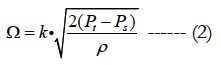
• Pt is the total pressure
• Ps is the static pressure
• ρ is the density of the flow
• Ω is the flow average velocity
• K is the flow coefficient: The flow coefficient of a device is a relative measure of its efficiency at allowing fluid flow. It describes the relationship between the pressure drop across an orifice, valve or other assembly and the corresponding flow rate.
• Cp is the flow pressure coffiecient
• Pinf is the free stream fluid pressure
• Qinf is the free stream fluid dynamic pressure: Dynamic pressure is the pressure on a surface at which a flowing fluid is brought to rest in excess of the pressure on it when the fluid is not flowing
• M designs the Mach number
• Γ is the ratio of the fluid heat capacities
• Z designs the altitude.
• T0 is the temperature in the standard conditions (T0 = 15°C).
• Mg0 is the gravitational force
• δT is the adiabatic thermal gradient.
• R is the constant for perfect gases.
• P0 is the pressure value in the standard conditions.
Pitot-Static Probe for Air Flow Velocity
Pitot-static probes for measuring aircraft speed and altitude are efficient instruments since their ability to provide a robust pressure measurement even on very particular conditions and properties of the surrounding flow as altitude, turbulence or density.
Mathematically, the conversion of the measurement pressure to a flow velocity measure is determined the following Bernoulli’s formula:
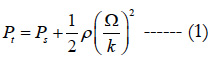
Once the total pressure, the static pressure and the density values are determined, one can conclude the average velocity:
As mentioned in the introduction section, the Pitot-static probe has two coaxial tubes that provide respectively the total and the static pressure. Figure 1 illustrates the standard design for measuring aircraft speed. On the basis of these measurement, the dynamic pressure, defined as the difference between the total pressure and the static one, is determined.
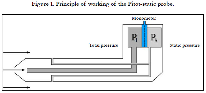
Figure 1. Principle of working of the Pitot-static probe.
The ISO Round Nose and the ISO tapered Nose are the most used designs for the Pitot-static probe head shapes. The choice of a tip design is based generally on performance/costs ratio.
Static pressure, is the pressure of a fluid at rest. Since the fluid is not moving, static pressure is the result of the fluid’s weight. The most common measurement method is to take the force exerted by the fluid and divide it by the area over which it is acting. Principle of how to measure the static pressure, is illustrated by Figure 2.
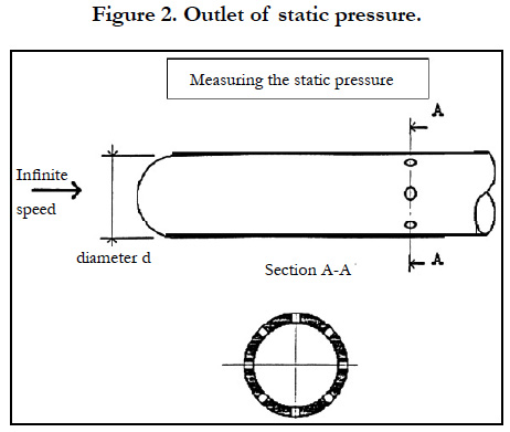
Figure 2. Outlet of static pressure.
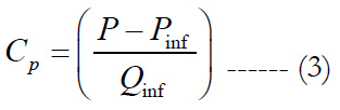
The pressure coefficient is a dimensionless number which expresses the ratio of pressure forces to inertial forces and permits to determine the suitable position of taking the static pressure measurement.
The pressure coefficient, noted Cp, can be expressed as:
The basic Pitot-static probe consists of a tube pointing directly into the fluid flow. As this probe contains fluid, a pressure can be measured; the moving fluid is brought to rest (stagnation) as there is no outlet to allow flow to continue.
The point where the flow stagnates is called the stagnation point. A small hole, placed on this tip and linked to a pressure transducer provides the total pressure measurement, also known as the stagnation pressure or (particularly in aviation) the Pitot pressure.
Figure 3 illustrates the different pressure measurements pick out in a Pitot probe.
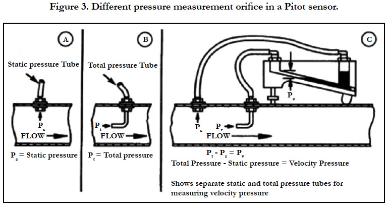
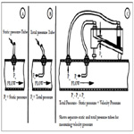
Figure 3. Different pressure measurement orifice in a Pitot sensor.
Main Factors of Measurement Inaccuracy
Factors that will therefore be taken into account in analysis of the Pitot tube failure: Air speed (Mach number), Altitude and Weather conditions (Temperature). The choice of these variable is justified with experimental and analytic proofs.
Many proposals have studied the influence of the disturbed flow on the used instrument measurement accuracy. For flows having a Mach number (M) over than 0.85, a local small shocks appear in the extremity of the probe which could disturb the sensor measurements [8].
The variation with Mach number of the static-pressure error ahead of fuselages with nose inlets has been determined from different shape tests [16] and flight scenario tests [17]. The results of the two tests given respectively by Figure 4 and 5, adapted from [16], show the same general variation of the error in the transonic speed range.
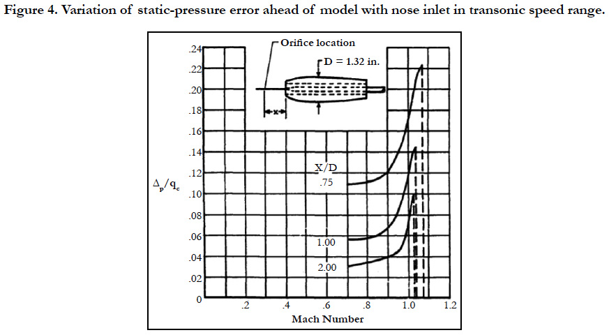
Figure 4. Variation of static-pressure error ahead of model with nose inlet in transonic speed range.
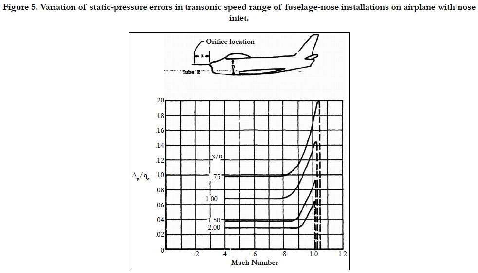
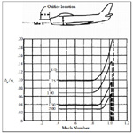
Figure 5. Variation of static-pressure errors in transonic speed range of fuselage-nose installations on airplane with nose inlet.
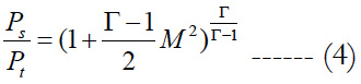
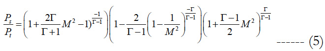
The relation between the Mach number and the static pressure is established mathematically by the two following equations:
For Mach < 1
For Mach > 1
Accurate information on speed and altitude parameters are essential to a safe and an efficient flight; speed measurements accuracy permits to well manage the aircraft at low speeds (stall condition) and to prevent critical situations of speeding, whereas accurate altitude measurements insures clearance of terrain obstacles and contributes in the aircraft balance maintain. The measurement accuracy issue for speed and altitude in the case of aeronautical applications has been the subject of a great many research investigations during the past five decades. The greater part of this research has been performed by a variety of organizations in Great Britain, Germany, and the United States. As an example, in the United States, investigations are conducted and leaded by government agencies (National Aeronautics and Space Administration (NASA). Since the flow density is a variable in the Bernoulli formula, the Pitot-static probe measurement depends on the flow density variations. In addition, a correction amount should be established at each speed measurement for each altitude. Since altitude and flow density are mathematically proportional, only one variable is chosen to be integrated in the model. In this study, we have chosen the altitude factor.
The barometric altitude (or pressure altitude) is the altitude deduced by taking only the static pressure surrounding the aircraft as a parameter.
In the troposphere, between 0 and 11 km altitude, the barometric altitude can be given by the following formula:
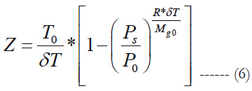
The derivative of The function (6) with respect to the variable Ps is :
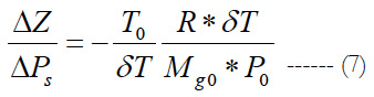
The variation of the static pressure is then a function of the variation of the altitude. In addition, it is necessary to take into account the altitude parameter in the static pressure variation analysis.
Temperature is considered as an important factor affecting the Pitot-static probes measurement accuracy during a flight because of the increasing risk of Pitot-static probe icing wich renders it incapable of performing its function of accurately sensing the flight velocity of the aircraft upon which it is mounted. Flight velocity is computed from dynamic pressure using the air density calculated from knowledge of the atmospheric temperature and the static pressure, as mentioned in the previous section; the temperature being measured independently. In a number of prior aircraft crashes, Pitot-static tube velocity readings are suspected as being incoherent due to icing and are believed to have lead to the crash. One example of a crash is the Air France Flight 447 in the 1 June 2009, believed to be due to ice collecting on or in one or more of the aircraft’s Pitot-static tubes during flight. For these reasons, temperature variable should be considered in the static pressure analysis since it presents an important environmental factor for the static tube functioning.
Factors Risk Analysis thought experimental plans application
The main purpose of this part is to study the effects of the covariates already defined on the above sections.
In addition, we propose the following algorithm:
Data acquisition consists in collecting the necessary information for the selected factors values in function of static pressure measurement error.
In this step, variables that impact on the measurement degradation of the studied equipment are determined. These factors should be then coded to facilitate their analysis through experiences plan. Factors coding is based on the following steps:
• When the influence factor is quantitative, the measurement values can be integrated directly into the model.
• When the variable is qualitative, it is recommended to use discrete values to quantify it. These values are associated with a scale defined by the modeller.
• For each factors values, the down level (minimum) and the up one (maximum) should be computed and mentioned.
The experiences plan matrix consists in a set of vectors where each one expresses the static pressure measurement error corresponding to the associated influencing factors values. These values are 1, for an up level or -1 for a down level.
At this stage, the key requirements are available to use the factorial regression analysis. From this data, the effect of each factor of influence on the static pressure measurement errors can thus be determined and discussed.
Data is extracted from research works on the static pressure measurement calibration, established by [15, 18] whose data is approved and certified by the NASA.
The influence factors have been already selected in the previous section. For each factor, we assign the value of 1 for up level and -1 for down level. These levels are determined as following for the three factors:
• Altitude: Up level = 35000 feet (ft), Down level = 0;
• Temperature: Up level = 40 Degree Celsius, Down level = -60 Degree Celsius;
• Mach number: Up level = 0.9, Down level = 0.2.
The Altitude and Temperature limit values are chosen based on International Civil Aviation Organization (ICAO) reports and the international Standard Atmosphere (ISA). The temperature at an altitude level of 35000 ft (nearly 11 Km), could reach -60°Celcius. Between 11 km and 20 km, the temperature remains constant.
On the basis of the defined levels of each factor (Step 2) and the data given in the Step 1, the experiences plan matrix is constructed. The table 1 illustrates this matrix on which our statistical analysis are built.
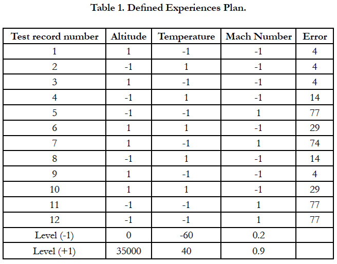

Table 1. Defined Experiences Plan.
The error column values in the Table 1 correspond to the values determined from the Data given by references [15] and [18]. These studies, approved by the NASA, determine the factors on which the Pitot sensor well-functioning depend and give results for measurement accuracy in function of different factors values.
On the basis of the above results shown in the three first steps, statistical results for the experiences plan are obtained. The first step of statistical analysis consists commonly in estimating the model significance. Table 2 illustrates the statistical results for the model were all defined variables are taken into account. In the first column, S designs the standard error of the regression and as the standard error of the estimate. S represents statistically the average distance that the observed values fall from the regression line. Conveniently, it highlights how wrong the regression model is on average using the units of the response variable. Smaller values are better because it indicates that the observations are closer to the fitted line. The second column provides the R-square which is a statistical measure of how close the data are to the fitted regression line. It is also known as the coefficient of determination, or the coefficient of multiple determination for multiple regression. Results of the table 2 are then interpreted to mean that the model fits the data (low S value) and is significant at 99.43 %.
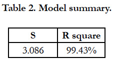
Table 2. Model summary.
The figure 6, indicates the significant terms on the basis of their P value. P values estimate the statistical significance, for each variable. The P variable involves the concept of likelihood, meaning the probability of the observed data being explained by the proposed regression model. The overall significance of each model is based on the ratio between the likelihood of a model in which the variables show no covariation with the survival time, and the likelihood of the standard model. Results shown by the figure 7 are interpreted to mean that the Altitude (A), Temperature (B), Mach Number (C) and Altitude * Temperature (AB) are significant. This conclusion can be also proofed by the analysis of variance results given in the table where the P value corresponding for each variable is less than 0.05 (the statistical significance threshold is fixed at 5%. A variable or a model is then significant if the corresponding P value is less than the error rate of 0.05).
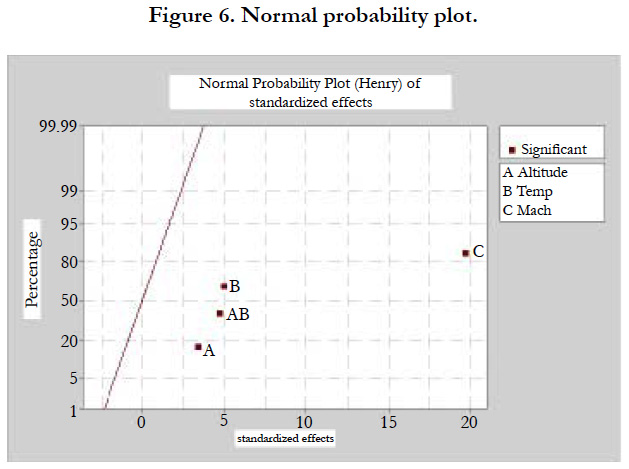
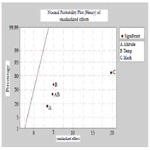
Figure 6. Normal probability plot.
In the table 3, the first column provides the sum of squares values, which design, for each variable, the measure of deviation from its mean. In statistics, the mean is the average of a set of numbers and is the most commonly used measure of central tendency. The arithmetic mean square given in the third column is simply calculated by summing up the square of values in the data set and dividing by the number of values. P values in the last column are already explained in the above analysis.
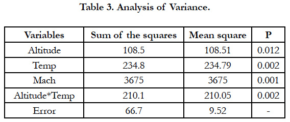
Table 3. Analysis of Variance.
Factor diagrams bring together the main effect graphs and interaction diagrams. A main effect is the change in the average response between two levels of factors. The chart of the main effects shows the averages for the Hours response with both order processing systems, as well as the averages for the Hours response with the two packing procedures. The interaction diagram shows the effects of the two factors, the order processing system and the packing procedure, on the response. Interaction occurs when the effect of one factor depends on the level of the other factor; so it is important to evaluate interactions.
In the figure 7, each point represents the average treatment time for a level of a factor. The horizontal center line indicates the average treatment time for all tests. The left pane of the chart indicates that measures that were taken with low altitudes where more efficient and precise than those taken with high altitude. The middle pane of the chart indicates that measures that were taken with low profiles of temperature had more precision than those taken with high temperature. The right pane of the chart indicates that measures that were taken with low number of mach of temperature had more precision than those taken with high number of mach. The figure highlights that the high effect of factors variation on the measurement precision is the effect of the Mach number, then the effect of the temperature and finally the effect of Altitude.
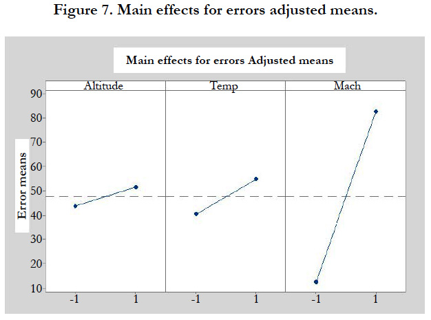
Figure 7. Main effects for errors adjusted means.
If there is no significant interaction between the factors, a graph of the main effects would correctly describe the relationship between each factor and the response. However, since the interaction is significant, you should also study the interaction diagram. A significant interaction between two factors can alter the interpretation of the main effects.
In the figure 8, each point in the interaction diagram represents the error means for static pressure measurement for a different combination of factor levels. If a two factors layouts are not parallel, it means that an interaction exists between the two considered factors. The interaction diagram indicates that the environment having a low temperature profile and high altitude have the most accurate measurement and then the lowest error mean (less than 20). Environment having a high temperature profile and high altitude have the least accurate measurement and then the highest mean error (nearly 65). Since the line corresponding to high temperature profile (red line) is more inclined, we can conclude that the high altitude has a greater effect on measurement precision when the surrounding environment has a high temperature profile instead of low one.
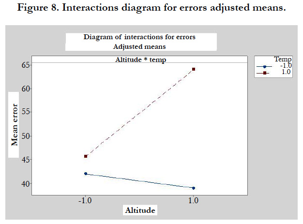
Figure 8. Interactions diagram for errors adjusted means.
Conclusions
This study deals with the Pitot static probe for aircraft application which, during a flight, is subject to internal and external conditions affecting its measurement accuracy. The first motivation of this paper is the empirical evidence to reduce accidents and fiight problems linked to Pitot-static probe malfunctioning. The aim of the first part of this paper is to collect and unify definitions for different parameters which impact the Pitot-static probe measurement accuracy. Parameters that has been chosen for failure mode analysis are Altitude, Temperature and Mach number. We have selected these parameters based on theoretical and experimental proposals which has dealt with the Pitot sensor working environment. Then, we have analyzed these factors statistically in order to highlight their real effect on the static pressure measurement value with experimental and mathematical investigations. Therefore, an algorithm based on experimental plans analysis is proposed for the defined factors to estimate numerically the real effect of each parameter.
References
- Cochran WG, Cox GM. Experimental designs. John Wiley and Sons: NewYork; 1950.
- Buckner RL, Bandettini PA, O’Craven KM, Savoy RL, Petersen SE, Raichle ME, et al. Detection of cortical activation during averaged single trials of a cognitive task using functional magnetic resonance imaging. Proc Natl Acad Sci USA. 1996 Dec 10;93(25):14878-83. PubMed PMID: 8962149.
- Mccarthy G, Luby M, Gore J, Goldman-Rakic P. Infrequent events transiently activate human prefrontal and parietal cortex as measured by functional MRI. J Neurophysiol. 1997 Mar;77(3):1630-4. PubMed PMID: 9084626.
- Werner FD, De LR, inventors; Rosemount Engineering Co Ltd, assignee. Static pressure probe. United States patent US 3120123A. Washington, DC: United States Patent Office; 1964 Feb 4.
- Pinckney SZ, inventor; National Aeronautics, Space Administration (NASA), assignee. Static pressure probe. United States patent US 3914997A. 1975 Oct 28.
- Miller DR, Comings EW. Static pressure distribution in the free turbulent jet. J Fluid Mech. 1957 Oct;3(1):1-6.
- Chigier NA, Beer JM. Velocity and static-pressure distributions in swirling air jets issuing from annular and divergent nozzles. J Basic Eng. 1964 Dec 1;86(4):788-96.
- Węcel D, Chmielniak T, Kotowicz J. Experimental and numerical investigations of the averaging Pitot tube and analysis of installation effects on the flow coefficient. Flow Meas Instrum. 2008 Oct 1;19(5):301-6.
- Bouhy JL. Evolution of the Pitot tube sensor. Journal A. 1991;32(3):83-6.
- Kalbfleisch JD, Prentice RL. The statistical analysis of failure time data. John Wiley & Sons; 2011 Jan 25.
- Box-Steffensmeier JM, Jones BS. Time is of the essence: Event history models in political science. Am J Pol Sci. 1997 Oct 1:1414-61.
- Dhillon BS. Failure modes and effects analysis--bibliography. Microelectron Reliab. 1992 May 1;32(5):719-31.
- Ower E, Pankhurst RC. The measurement of air flow. Elsevier; 2014 May 9.
- Miller RW. Flow measurement engineering handbook. Instrument Society of America: Research Triangle Park, NC; 1983.
- Gracey W. Measurement of aircraft speed and altitude. National Aeronautics and Space Administration Hampton Va Langley Research Center; 1980 May.
- Gracey W. Survey of altitude-measuring methods for the vertical separation of aircraft. National Aeronautics and Space Administration; 1961.
- Expendable Pressure Sensor Rocketsonde - Phase I. Rep. No. 1329 (Contract AF 33(600)-37984). Bendix Aviation Corp;1959 Oct 15.
- DeAnda AG. AFFTC Standard Airspeed Calibration Procedures. Air Force Flight Test Center Edwards AFB CA; 1981 Jun.