Rotating Flow Simulations with OpenFOAM
Wilhelm D*
Zurich University of Applied Sciences, Institute of Applied Mathematics and Physics, Techikumstrasse 9, 8400 Winterthur, Switzerland.
*Corresponding Author
Dirk Wilhelm,
Zurich University of Applied Sciences,
Institute of Applied Mathematics and Physics,
Technikumstrasse 9, 8400 Winterthur, Switzerland.
E-mail: wilk@zhaw.ch
Article Type: Review Article
Received: July 16, 2015 ; Accepted: September 28, 2015; Published: October 06, 2015
Citation: Wilhelm D (2015) Rotating Flow Simulations with Open-FOAM. Int J Aeronautics Aerospace Res. S1:001, 1-7.
doi: dx.doi.org/10.19070/2470-4415-SI01001
Copyright: Wilhelm D© 2015 This is an open-access article distributed under the terms of the Creative Commons Attribution License, which permits unrestricted use, distribution and reproduction in any medium, provided the original author and source are credited.
Abstract
Rotating flow problems have a wide range of applications in several technical fields, e.g. gas turbines, water turbines, wind turbines, aircraft engines, chemical engineering, process engineering, or medical devices. Computational fluid dynamics (CFD) has gain significant importance for the physical analysis and mechanical design of rotating flow systems. Beside commercial tools open source tools like openFOAM have become more and more accepted in academia and also in industry in the last years. In the present paper, we discuss the treatment of rotating flow systems in general and focus especially on openFOAM simulations. The distinction between Single Reference Frame (SRF) and Multi Reference Frame (MRF) simulations is explained for steady and unsteady flow problems. In particular the handling of interfaces between fixed and rotating flow regions is discussed. The purpose of the present paper is, to give an overview of the different techniques available in openFOAM for simulation of rotating flow problems. It is stated that unsteady flow simulations are much more time consuming compared to frozen rotor simulations or mixing plane techniques. Consequently, steady-state simulation techniques should be considered, whenever a steady-state physical flow field solution is expected.
2 Methodology and Results
2.1. Single Reference Frame
2.2. Simulation of Gas Bearing System
2.3 Multi Reference Frame
2.4 Mixing plane approach
3.Discussion
4.Conclusion
5.References
Introduction
Many aerodynamic, hydrodynamic, and especially turbomachinery applications are conducted in rotating flow regimes, see e.g. [1- 3]. Beside experimental measurements Computational Fluid Dynamics (CFD) simulations play an increasing role for analysis and design of such fluid flow problems. For instance turbomachinery design has been strongly supported by CFD. First, CFD has been employed as flow analysis tool and over the last decades it has been more and more integrated in the design process of turbomachinery. The benefit ranges from shorter design cycles over cost reduction to performance optimization. For a general overview of CFD application in turbomachinery see e.g. [4-8].
Several commercial CFD tools are widely-used in industry and academia, like Star CCM+ [9] ANSYS Fluent [10] or ANSYS CFX [11]. These tools offer a wide range of functionalities for the simulation of varies fluid flow problems, including rotating flow problems, and turbomachinery applications. However, commercial codes have rather high purchase costs and are also expensive in operation and maintenance. Therefore, open source solutions have become more and more popular in recent years. One of these open source CFD tools is OpenFOAM (see e.g. [12, 13]) that has been developed to a powerful tool for the simulation of a wide range of flow problems [14]. Among these are rotating flow applications in various fields.
OpenFOAM has been employed e.g. for the simulation of the Ercoftac centrifugal pump case by Petit et. al. [15]. Nilsson and Cervantes [16] analyzed the Turbine-99 Kaplan draft tube and compared the OpenFOAM simulation results with ANSYS CFX results and experimental measurements. The authors showed fairly good agreement between the two simulation codes. However, discrepancies between simulations and measurements were found that are due to differences in the measured phased-averaged and time-averaged inflow data [16]. Bounous [17] analyzed the ERCOFTAC conical diffuser with openFOAM studying cases with different boundary conditions and turbulence models (k-ε,k- ω-SST). Koch et al. [18] employed OpenFOAM for the simulation of a high speed micro turbine for bio-medical applications.
For the modeling of complex flow systems containing rotating parts specific numerical approaches are needed. Various techniques have been developed in the past (e.g.[19-22]) to account for the rotation effects on the fluid. The purpose of the present work is to give in a mini-review a deep insight in the methodology of rotating flow simulation. It will be presented how rotating flows are numerically modelled in general and especially with the openFOAM simulation tool.
Methodology and Results
Rotating flow problems may be distinguished between steady and unsteady flows. Moreover, Single Reference Frame (SRF) and Multiple Reference Frame (MRF) methods are usually employed. Table 1 gives an overview of the openFOAM solvers for the different flow cases. In contrary to the SRF method, which is only suitable for one single rotating domain, where the complete computational fluid region is in motion, the MRF approaches enables the possibility to simulate two or more domains which of them may be either stationary or in motion.
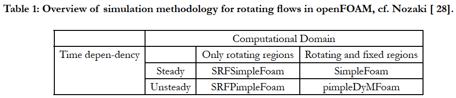

Table 1: Overview of simulation methodology for rotating flows in openFOAM, cf. Nozaki [28].
The connection between the different regions is handled by a mesh interface. Arbitrary Mesh Interfaces (AMI) are commonly used in this context. Herein, the interface between the stationary and the rotation part of the computational geometry is required exclusively for the numerical simulation and has no physical meaning.
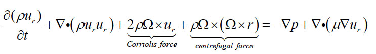
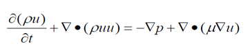
For a rotating (non-inertial) coordinate system on the rotor the flow is usually steady relative to the rotating frame. The MRF method is mostly used to simulate such steady state-flow problems. The Navier-Stokes equations are solved in a relative frame.
Single Reference Frame
A good example for a steady-state single rotating flow region problem is the Couette flow (see Figure 1), where the entire flow regime is confined between two rotating cylinders. The twodimensional Couette flow is steady, but it develops the Taylor instability for increasing Taylor number.
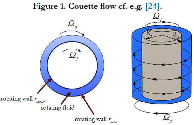
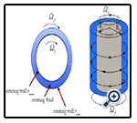
Figure 1. Couette flow cf. e.g. [24].

This instability leads to the three-dimensional Taylor flow (see Figure 2). Hence, the Couette flow can be simulated with the steady-state SRF SimpleFoam solver module of openFOAM. However, the Talyor instability has to be treated with an unsteady solver, e.g. the SRFPimpleFoam module. The SRF SimpleFoam solver utilizes the SIMPLE algorithm for decoupling of the momentum equation and the continuity equation ([26, 27]) yielding a steady-state fluid flow solution. The SRF PimpleFoam uses PIMPLE algorithm [26] to solve the unsteady rotating flow problem.
Figure 2. Taylor-Coutte flow. Left: sketch, right: contours of instantaneous azimuthal velocity, reprinted form [29] with permission form Cambridge University Press.
For the openFOAM version 2.3.0, the tutorial of a mixer is very instructive to get used to the SRF SimpleFoam solver. The tutorial is given in the source code under: Tutorials/incompressible/SRF Simple Foam/mixer:
It solves the flow in a segment of a rotating mixer with a given angular velocity of 5000 rpm. The flow geometry shown in Figure 3 exhibits outerfixed wall, inner rotating wall with rotating blades, and periodic boundary in azimuthal direction. The inlet and outlet boundaries are perpendicular to the rotation axis (i.e. we have an axial turbomachinery system). Due to periodicity in the azimuthal direction, only a segment of 90° is considered for the simulation.
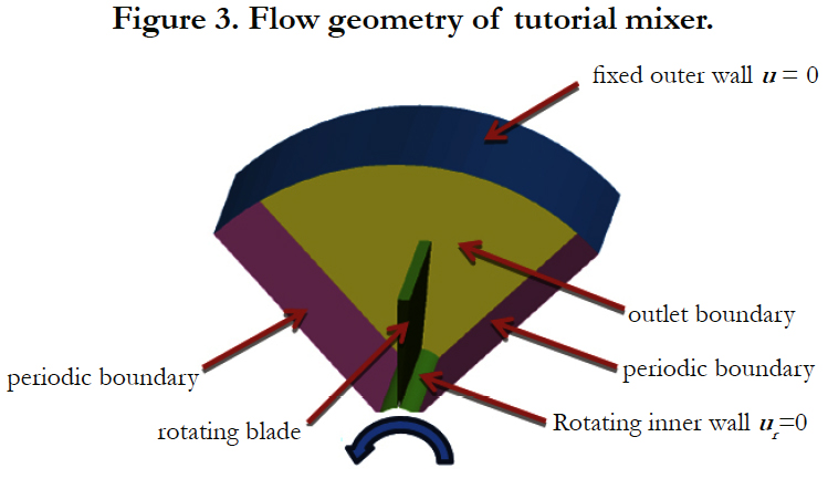
Figure 3. Flow geometry of tutorial mixer.
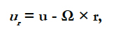
OpenFOAM provides the possibility to solve for the relative velocity ur in the rotating reference frame. Figure 4 shows the relative and absolute velocity after 1000 time steps of 1 sec each. It is clearly seen that the velocity at the outer wall is vanishing in the fixed frame of reference and in the rotating frame the relative velocity is ur = u - Ω × r, i.e. |ur|=51.36 m/s. Here the angular velocity is Ω=5000 rpm=5000 2π/60=523.6 rad/s and the outer radius is r =0.1m.
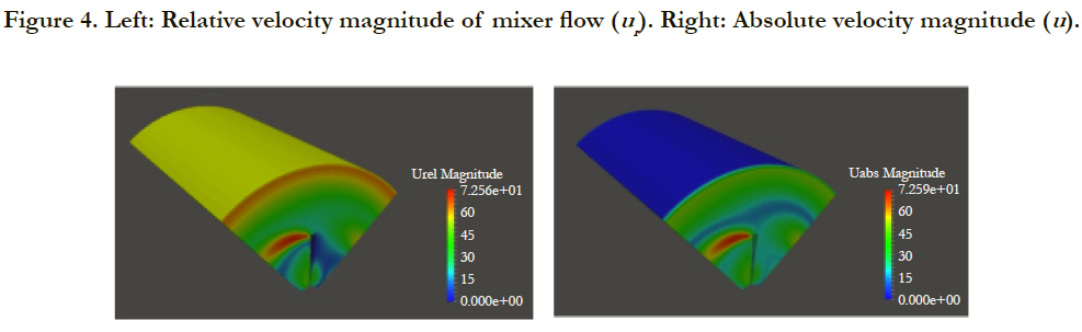
Figure 4. Left: Relative velocity magnitude of mixer flow (ur ). Right: Absolute velocity magnitude (u).
Simulation of Gas Bearing System
In [30] we simulated a micro turbine that is employed in a Nuclear Magnetic Resonance (NMR) system. Nuclear Magnetic Resonance (NMR) is a widely used technique for chemical and biological analysis (e.g. [31-33]). The micro turbine has a diameter of 1.3mm and is rotating very fast with up to 67’000 revolutions per second. It consists of Pelton type turbine blades and is driven by an air gas flow. Figure 5 shows the geometry of the NMR micro turbine system that is lubricated by radial air bearings.
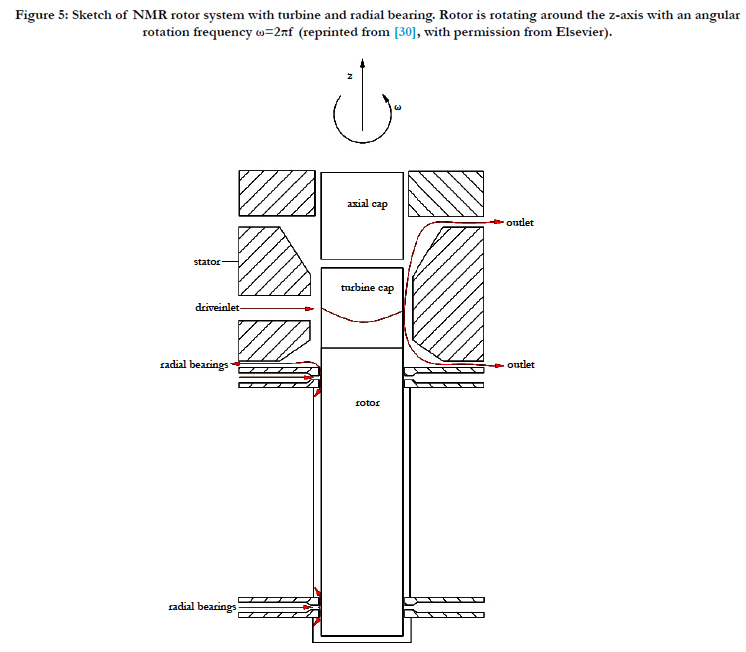
Figure 5: Sketch of NMR rotor system with turbine and radial bearing. Rotor is rotating around the z-axis with an angular rotation frequency ω=2πf reprinted from [30], with permission from Elsevier.
In the present work, we will consider a simplification of such an air bearing system. Figure 6 shows the flow geometry with inflow and outflow boundaries. For simplicity, only a quarter of the entire flow domain is simulated and periodic boundary conditions are imposed in circumferential direction. An inflow velocity boundary condition of vin=100m/s is prescribed at the inlet in Figure 6. Here we skipped the inlet pipe with the nozzle which allows for a significant reduction of the current flow case. Consequently, a single reference frame with one rotating domain can be employed. Note that the main challenge for this approach is the definition of the appropriate boundary condition at the inlet. In the present case, we approximated the inlet velocity from the inlet pressure that is prescribed at the actual inlet of the flow geometry. To overcome the problem, often a multi reference frame with a steady flow domain in the pipe and a rotating flow domain in the bearing is employed. However, the single reference frame approach has the clear advantage that parameter studies can be conducted very efficient. For example the loads of the bearing as function of inlet velocity for different eccentricities are important parameters for a characterization of the bearing.
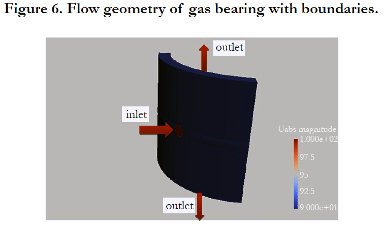
Figure 6. Flow geometry of gas bearing with boundaries.
The rotation frequency is set to f=10000 Hz (i.e. 10000 revolutions per second). Radial gap between the rotor and the outer cylinder support is d=0.1mm. The velocity streamlines given in Figure 7 clearly show the propagation of the inlet fluid in the rotation direction. In Figure 7 the velocity and pressure are depicted in a cut through the inlet of constant z-position showing the high relative velocity in the region close to the inlet hole. The aim of the numerical simulation studies is the optimization of the stability behavior of the gas bearing, since the rotation frequency of several kHz is far above the lower unstable modes of the system. These optimizations will be conducted in future simulation studies.
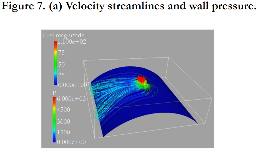
Figure 7. (a) Velocity streamlines and wall pressure.
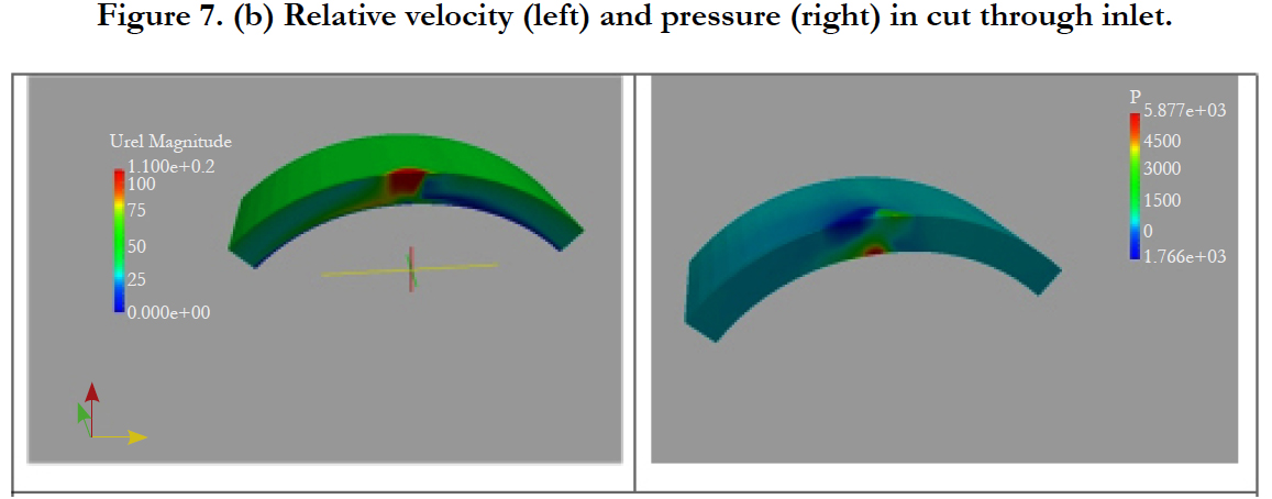
Figure 7. (b) Relative velocity (left) and pressure (right) in cut through inlet.
Multi Reference Frame
The most rotating flow applications involve steady and unsteady flow regions. Good examples are turbomachinery applications of rotor stator systems like axial gas turbines. Figure 8 shows an aircraft turbine (J85-GE-17A) and the sketch of the rotor stator system. The stator ‘S’ is fixed and the rotor ‘Sch’ is rotating with a given angular velocity Ω. In Figure 8 the computational domain can be decomposed in one subdomain (between positions 1 and2) linked to a fixed frame of reference and a second subdomain (between position 2 and 3) linked to a rotating frame of reference. The two domains are connected by a sheared interface ‘I’.
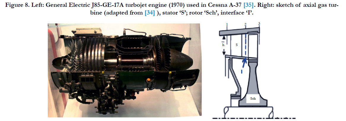
Figure 8. Left: General Electric J85-GE-17A turbojet engine (1970) used in Cessna A-37 [35]. Right: sketch of axial gas turbine (adapted from [34] ), stator ‘S’; rotor ‘Sch’, interface ‘I’.
The information between different zones (stationary and rotating) is transferred through an Arbitrary Mesh Interface (AMI), i.e. interface I in Figure 8, at each iteration step. At these interfaces between the two references frames a velocity steady-state flow condition is applied which assumes the same absolute velocity on both sides of the interface and therefore for each reference frame. The challenge of the MRF method is the appropriate positioning of the interfaces in the geometry and the generation of a consistent mesh for both sides of the interface. Although the meshes at the interfaces do not have to match perfectly due to the AMI approach a similar and uniform cell size on both sides can significantly increase the accuracy of the results. Figure 9 shows the principle of an AMI for a meshed fixed domain (stator) and a moving domain (rotor).
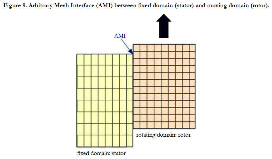
Figure 9. Arbitrary Mesh Interface (AMI) between fixed domain (stator) and moving domain (rotor).
In openFOAM version 2.3.0 the tutorial of mixer vessel unsteady flow problem is given in the source code in: incompressible/ pimpleDyMFoam/mixerVesselAMI2D.
It consists of an inner rotating domain (mixer) and an outer static domain (stator), see Figure 10. The two subdomains are separated by an AMI and the simulation is performed with the PIMPLE solver pimpleDyMFoam. Figure 10 shows the velocity magnitude of the mixer problem after 100 time steps with time step Δt=1/1000sec.
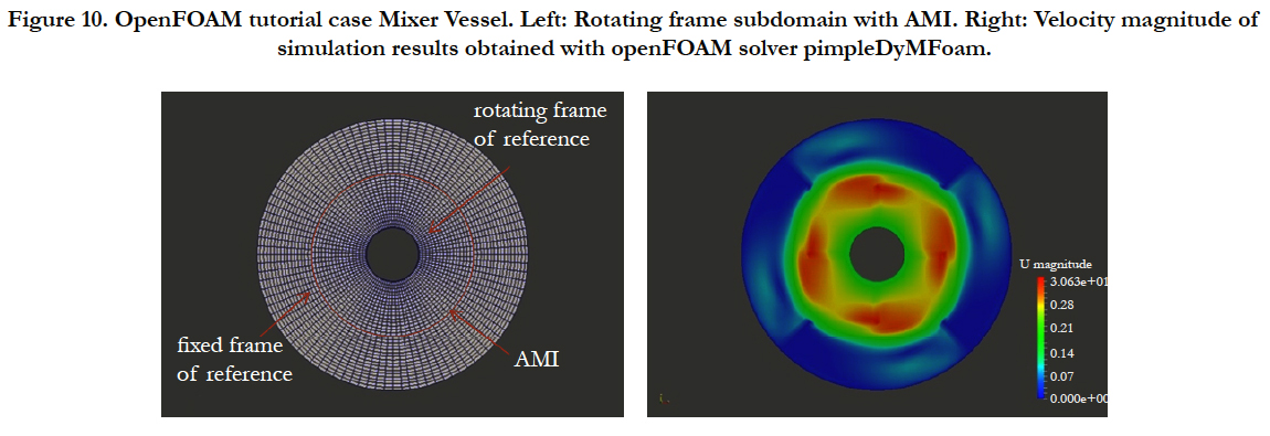
Figure 10. OpenFOAM tutorial case Mixer Vessel. Left: Rotating frame subdomain with AMI. Right: Velocity magnitude of simulation results obtained with openFOAM solver pimpleDyMFoam.
Mixing plane approach
The pimpleDyMFoam has the disadvantage that unsteady simulations are very time consuming. The mixing plane technique is common for steady-state simulation of multi domain problems, e.g. multi-row systems in a gas turbine. Herein the variables at the interfaces between rotating and fixed parts are circumferential averaged. In Figure 8 the interface at position 2 between the rotor and stator can be described by a mixing plane. In this case the equations are separately solved first in the rotor domain and afterwards in the stator domain, employing the mixing plane as boundary for each iteration step. Note that this method does not treat the rotor-stator interaction correctly, because it is an unsteady phenomenon and the main structure of the flow will be lost during the averaging process. Nevertheless, it is a feasible way of getting steady-state solutions of multi-row problems and it provides a suitable representation of the flow problem. In OpenFOAM the following tutorial can be found for simulation of an axial turbine with mixing planes.
foam-extend-3.1/tutorials/incompressible/MRF SimpleFoam/axialTurbine_mixingPlane
Discussion
OpenFOAM and many other CFD simulation tools provide different functionalities to handle rotating flow problems. It has to be distinguished, if only one rotating flow domain is considered or several fixed and rotating domains. Single Reference Frame (SRF) simulations can be performed to very low costs and are therefore predestinated for elaborated multi parameter studies. The Multi Reference Frame (MRF) approach is the common casein turbomachinery and most other applications of rotating flow systems. If we consider two subdomains one static (e.g. a stator of an axial turbine) and one rotating (e.g. the rotor of an axial turbine), the governing flow equations can be solved independently, when proper conditions are prescript at the internal interface between the two domains. We distinguish the following cases:
- Frozen Rotor Technique: Is a steady-state simulation that solves the equation for one rotor position and converges to a snapshot of the fluid flow system. The simulation runs are normally very fast. In some cases it is advantageous to conduct the simulation at several rotor positions and average integral quantities. For openFOAM this method employs the SIMPLE solver algorithms.
- Sliding Mesh Method: Is used for unsteady simulations. The sliding mesh method allows adjacent grids to slide relative to each other along the internal interface surface, whereas the coupling between the two regions is achieved by interpolating the flow variables on the cell faces. For openFOAM, this method employs the PIMPLE solver to obtain an unsteady solution, which has the disadvantage of much larger computational time than the frozen rotor technique.
- Mixing Plane Approach: Is employed for steady-state simulations of MRF systems. It provides a circumferential average of all flow quantities in the internal interface (the mixing plane). This approach gives a better approximation of the steady-state flow than the Frozen Rotor Technique and is much less computational time consuming than the unsteady simulation approach. However, local flow information, like local vortices are smeared out over the mixing plane, hence the results represent only an averaged state and not a snapshot or a physical time step.
Conclusion
The present paper gives an overview of the different techniques for the simulation of rotating flow problems, which have widespread applications for example in turbomachinery, hydrodynamics or aerodynamics. The differences between Single Reference Frame (SRF) systems and Multi Reference Frame (MRF) systems are discussed. Furthermore, the different techniques for the simulation of steady-state or unsteady flow problems are presented. The different cases are discussed specially for the openFOAM software tool, but are of general relevance for various CFD tools.
Acknowledgement
This work was supported by the Commission for Technology and Innovation in the framework of the project KTI-Nr. 17247.1 PFIW-IW.
References
- Bohl W, Elmendorf W (2012) Strömungsmaschinen 1,Vogel, Würzburg, Germany.
- White MW (2016) Fluid Mechanics, McGraw-Hill Education, New York, USA.
- Dixon SL, Hall CA (2014) Fluid Mechanics and Thermodynamics of Turbomachinery, Butterworth Heinemann, Boson, USA.
- Denton JD, Dawes WN (1998) Computational fluid dynamics for turbomachinery design, Proceedings of the Institution of Mechanical Engineers, Part C: Journal of Mechanical Engineering Science 213(2): 107-124.
- Horlock JH, Denton JD (2005) A review of some early design practice using computational fluid dynamics and a current perspective. J Turbomach 127: 5-13.
- Chen N (2010) Aerothermodynamics of Turbomachinery: Analysis and Design. John Wiley & Sons, Singapore.
- Logan E, Roy R (2003) Handbook of Turbomachinery. Marcel Dekker Inc., USA.
- Hawthorne WR, Novak RA (1969) Aerodynamics of turbo-machinery. Annu Rev Fluid Mech 1: 341-366.?
- Star CCM+ http://www.cd-adapco.com/products/star-ccm.
- ANSYS Fluent http://www.ansys.com/Products/Simulation+Technology/Fluid+Dynamics/Fluid+Dynamics+Products/ANSYS+Fluent.
- ANSYS CFX http://www.ansys.com/Products/Simulation+Technology/Fluid+Dynamics/Fluid+Dynamics+Products/ANSYS+CFX.
- https://openfoamwiki.net/index.php/OpenFOAM_guide.
- http://www.openfoam.org/.
- OpenFOAM Workshop (2015) Ann Arbor, Michigan, USA.
- Petit O, Page M, Beaudoin M, Nilsson H (2009) The ERCOFTAC centrifugal pump OpenFOAM case-study. 3rdIHAR International Meeting of the Workgroup on Cavitation and Dynamic Problems in Hydraulic Machinery and Systems, Brno, Czech Republic.
- Nilsson H, Cervantes M (2012) Effects of inlet boundary conditions, on the computed flow in the Turbine-99 draft tube, using OpenFOAM and CFX. 26th IAHR Symposium on Hydraulic Machinery and Systems, In: IOP Conf. Series: Earth and Environmental Science 15.
- Bounous O (2008) Studies of the ERCOFTAC conical diffuser with OpenFOAM. Department of Applied Mechanics Chalmers University of technology, Göteborg, Sweden.
- Koch S, Herzog N, Wilhelm D, Purea A, Osen D, et al. (2015) Aerodynamic optimization of a micro turbine inserted in MAS systems, in preparation.
- Gosman AD (1998) Developments in Industrial Computational Fluid Dynamics. Chem Eng Res Des 76(2): 153-161.
- Issa RI, Sadri MA (1998) Numerical Modeling of Unsteady Flow through a Turbomachine Stage. ASME 98-GT-253.
- Hillewaert K, van den Braembussche R (2000) Comparison of Frozen Rotor to Unsteady Calculations of Incompressible Turbomachinery Flow. In Proceedings of the 5th National Congress on Theoretical and Applied Mechanics, Louvain-la-Neuve 335-338.
- Hirsch C (1989) Numerical Computation of Internal and External Flows. vols. 1 and 2, John Wiley & Sons, Chichester, UK.
- Graebel WP (2007) Advanced Fluid Mechanics. Elsevier, Amsterdam, Netherlands.
- Landau LD, Lifschitz EM (1991) Hydrodynamik. Akademie Verlag, Berlin, Germany.
- Ostilla R, Stevens RJ, Grossmann S, Verzicco R, Lohse D (2013) Optimal Taylor-Couettefow: direct numerical simulations. J Fluid Mech 719: 14-46.
- Ferziger JH, Perić M (2002) Computational Methods for Fluid Dynamics. Springer-Verlag, Berlin, Germany.
- Jasak H (1996) Error Analysis and Estimation for the Finite Volume method with Applications to Fluid Flows. Ph.D. Thesis, Imperial College of Science, Technology and Medicine, London, UK.
- Nozaki F (2014) CFD for rotating machinery using openFOAM v2.3.0. http://de.slideshare.net/fumiyanozaki96/cfd-for-rotating-machinery-usingopenfoam.
- Dong S (2007) Direct numerical simulation of turbulent Taylor–Couette flow. J Fluid Mech 587: 373-393.
- Wilhelm D, Purea A, Engelke F (2015) Fluid flow dynamics in MAS systems. J Magn Reson 257: 51-63.
- Ernst R, Bodenhausen G, Wokaun A (1989) Principles of Nuclear Magnetic Resonance in One and Two Dimension. Oxford University Press, New York,USA.
- Keeler J (2007) Understanding NMR Spectroscopy. John Wiley and Sons, Chichester, England.
- Blümich B (2005) Essential NMR: For Scientists and Engineers. Springer-Verlag Berlin Heidelberg, Germany.
- Rick H (2013) Gasturbinen und Flugantriebe. Springer Vieweg, Berlin, Germany.
- Acharya S (2008) Wikipedia https://en.wikipedia.org/wiki/Acharya_S.