Comparison of Various Methods for Orbital Measurements Processing
A.I. Nazasrenko*
Professor, Chief Scientist, Scienific Technological Center, "KOSMONIT", RosCosmos, Russia.
*Corresponding Author
A.I. Nazasrenko,
Professor, Chief Scientist, Scienific Technological Center,
"KOSMONIT", RosCosmos, Russia.
Tel: 8499 187 02 68
Email: anazarenko32@mail.ru
Received: March 20, 2019; Accepted: April 02, 2019; Published: April 05, 2019
Citation: A.I. Nazasrenko. Comparison of Various Methods for Orbital Measurements Processing. Int J Aeronautics Aerospace Res. 2019;6(3):180-184. doi: dx.doi.org/10.19070/2470-4415-1900021
Copyright: A.I. Nazasrenko© 2019. This is an open-access article distributed under the terms of the Creative Commons Attribution License, which permits unrestricted use, distribution and reproduction in any medium, provided the original author and source are credited.
Abstract
The application of joint measurements processing in updating satellite orbits faces the necessity of correct accounting for random perturbations. In the early 70-ies it was suggested to improve the least square technique (LST) based on accounting for random perturbations in "weighing" the measurements. This improvement was called the method for Optimal Filtration of Measurement (OFM).
The comparison of the accuracy of estimates, obtained with using the LST (with extension and without extension of the state vector), as well as the OFM method, was performed. It was shown that, in the presence of perturbations, the application of the OFM method provides the best accuracy.
2.Abbreviations
3.Introduction
4.Brief Information on the Method of Optimal Filtration of Measurements
5.Comparative Analysis of Errors
6.Conclusion
7.References
Keywords
Least Square; Random Perturbations; Optimal Filtration.
Abbreviations
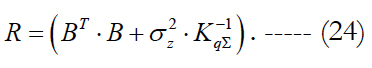
LST: Least Square Technique; OFM: Optimal Filtration of Measurement.
Introduction
The Least Square Technique is traditionally used for determining (updating) orbital parameters based on measurements [1, 2]. This technique was developed 200 years ago, when there were no artificial satellites yet. A typical feature of motion of nearearth artificial satellites is the essential effect of disturbing factors, which cannot be described mathematically to a required accuracy. A typical example of such disturbances is the atmospheric drag, whose value is proportional to the product of a real ballistic factor by the atmospheric density. The main difficulty arising in accounting for these factors at prediction consists in their unpredictable time variation.
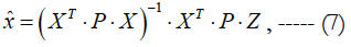
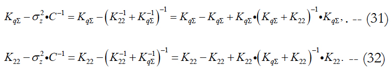
In using LST, the effect of disturbing factors is manifested in the necessity of choosing the so-called optimum fit span, i.e. the time interval over which the used measurements are located. The dependence of errors of estimations with using LST on the fit span value is presented schematically in Figure 1. The studies have shown that the optimum value depends not only on the drag value, but on the accuracy of measurements and on their quantity as well. In practice, this interval is usually determined from experience and is specified to be constant for particular types of satellites.
The dashed line relates to the case of absence of perturbations (the ideal LST). The bold line shows the dependency you want to get as a result of updating the data processing techniques in the presence of random perturbations.
So, when using the least square technique the achieved level of errors in determination and prediction of orbits is stipulated by the influence of unpredictable perturbations over the data processing interval and at prediction, as well as by the impossibility of correct accounting for these perturbations.
Let us pay attention to the recurrence techniques for processing the measurements [2, 3], which take into account the effect of system’s noise (white or colored). These techniques make it possible to process the measurements successively. As a result, the processing accuracy increases. In Figure 1 their characteristics are marked as "Updating". However, the experience of application of recurrent algorithms revealed their following disadvantages:
- The sensitivity to the accuracy of a priori characteristics of system’s noise. Naturally, these a priori data always differ from the real noise characteristics. This discrepancy leads to possible increasing of errors (divergence in the updating process) with increasing the fit span length. Such a possibility is shown in Figure 1 by a dotted line.
-The recurrent nature of the algorithm, where the previous measurements are not stored, impedes providing high reliability of its operation in the cases of coming abnormal measurements.
- The admission of a linear nature of correlations between the measurements and a state vector represents a simplification, because the initial equations are nonlinear for satellites. In the absence of previous measurements, the use of iterations for accounting the nonlinearity occurs to be ineffective.
In the 70-ies and 80-ies, the use of a recurrent data processing algorithm was an involuntary measure in the conditions of massive calculations. With limited characteristics of computer technology at that time, this measure made it possible to considerably reduce the time interval between successive refinements of the elements of orbits for each satellite, and, thus, to increase their accuracy at the current time instant. In subsequent years, with improving computer technology performances, it became possible to pass to joint processing of measurements with updating the elements of orbits of all satellites, i.e. to application of the LST and its modifications.
The application of joint processing of measurements with updating the satellite orbits faces the necessity of correct consideration of random perturbations. If the latter ones are not taken into consideration (as in the classic LST), one needs to limit the fit span (see Figure 1). In this case, we do not use the available reserves of increasing the accuracy that have been demonstrated by recurrent algorithms (the "Updating" curve in Figure 1).
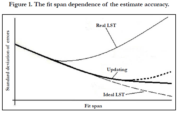
Figure 1. The fit span dependence of the estimate accuracy.
In the early 70-ies, it was suggested to improve LST based on accounting for random perturbations [3]. In subsequent works (Nazarenko, 1998, 2007, 2009, 2010, 2013, 2015; Nazarenko et al, 2007) [4-11] this approach was updated and got the name of the method for Optimal Filtration of Measurements. The prominent feature of the developed technique is accounting for statistical characteristics of atmospheric disturbances on a fit span and during the motion prediction.
Brief Information on the Method of Optimal Filtration
of Measurements
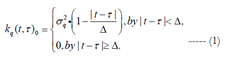
According to paper (Nazarenko, 2015) [10], the autocorrelation function of atmospheric disturbances is assumed to be of the form:
The initial data for applying this correlation function are:
ΔT - the change of the period under an effect of atmospheric drag per revolution, which is calculated on the basis of numerical integration with the mean value of ballistic coefficient;
katm - the RMS of random atmospheric disturbances with respect to their mean value;
Δ - the interval of correlation of atmospheric disturbances.
The first two quantities are used for calculating the RMS of atmospheric drag variations according to the formula:
The matrices of cross-correlation of errors in forecasting the state vector at time instants (ti and tl) are calculated according to the formula:

where
Here tk is time of updating the state vector x, U(ti, ξ) is the socalled transition matrix of dimension (6x6), F(ξ) is the matrix of coefficients at atmospheric drag in the differential equations of the disturbed motion.
In the OFM technique, the problem of evaluating the state vector x (n×1) based on the measurements Z (k×1) is considered in the classical formulation. The possibility of existence of some interfering parameters q (m×1) is taken into consideration. In this case, the basic initial relationship for measurements Z takes the form:
Here X (k×n) and B (k×m) are the known matrices, V (k×1) is the vector of errors in measurements, which are assumed to be equally accurate and statistically independent variables, i.e.
Note. In general, errors in measurements are not equally accurate and statistically independently. However, we do not consider this case because it would complicate the conversion but did not affect the main results.
The correlation matrix of interfering parameters M(q∙qT)=KqΣ=σ2 q∙Kq is assumed to be known. It is constructed taking into account the correlation of atmospheric disturbances (1) and is used for “weighing” the measurements without expanding the state vector. The effect of interfering parameters is taken into consideration by their combining with the errors of measurements (VΣ=B∙q+V), and then the maximum likelihood technique is applied. In this case, the required estimate is expressed as follows:
where
Here parameter Sn can be treated as the signal-to-noise ratio. The estimate (7) provides the minimum of the criterion:
The feature of estimate (7) is the fact that it is suitable for any time instants, including forecasting one. The value of interfering parameters (noises) is calculated after constructing the estimate (7) on the basis of residual discrepancies with using the relationship of the form
where F(t) is some matrix.
Another feature of the OFM technique is the necessity in the inversion of matrix (8) of dimension (k×k). With contemporary characteristics of computer technology, this operation is quite feasible.
The consideration of atmospheric disturbances in updating the orbits is manifested in a substantially different (as compared to the Least Square Technique) behavior of residual discrepancies between the measured and updated orbital parameters over the fit span. The physical sense of this effect lies in the fact that the initial measurement data are not "spread" uniformly, but are concentrated in the vicinity of the last point of a fit span.
Comparative Analysis of Errors
Consider the problem of estimating the state vector x (n×1) based on measurements Z (k×1) in the classical formulation. We take into account the possibility of existence of certain interfering parameters q (m×1). In this case, the main source ratio has the form (5).
The comparative characteristics of the OMF technique accuracy were published in a rather general form in paper and in the monograph [7, 8]. Here we will discuss them in more details. Three approaches to the state vector estimation were considered, which differ in the method of accounting for interfering parameters (such as the atmospheric drag):
1. Without accounting for interfering parameters. The effect of interfering parameters is not taken into account in the process of state vector estimation. In this case, the classical method of least squares is used:
It is easy to show that the correlation matrix of the vector of errors is expressed as follows:

2. Parameterization. The vector of interfering parameters is introduced into the composition of the extended state vector yT = ||x, q||T, and then the LST is applied. In this case, the desired estimate and its correlation matrix are expressed as follows:
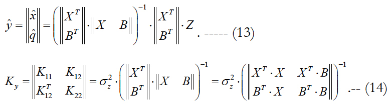
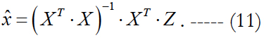
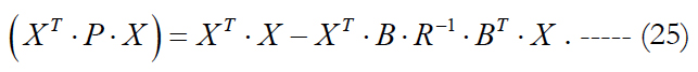
Now we perform the comparison of estimates (12) and (14). We will use the methodology of inversion of block matrices and, in particular, the Frobenius formula. Then the right-hand side of equation (14) can be expressed as follows:
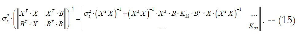
Here the correlation matrix of noise errors is equals to:
With accounting for formula (14), it follows from (15) that in this case (when we extend the state vector) the correlation matrix of the state vector x is equal to:

The form of this expression is useful for comparison with formula (12) for the correlation matrix of errors, when the LST is applied directly without extending the state vector. Let us express the difference of estimates (12) and (17). We get:

It is obvious from this expression, that, if the difference (KqΣ - K22) is a positively defined matrix, i.e., if the condition:
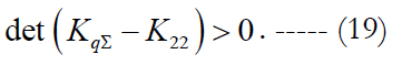
is met, then the transition to technology II (Parameterization) leads to increasing the accuracy of estimates as compared to the LST without extending the state vector. Otherwise, the LST application without extending the state vector will provide a higher accuracy.
Note. Condition (19) represents the generalization of a similar condition for the partial (scalar) case, which was substantiated in the author’s article [11].
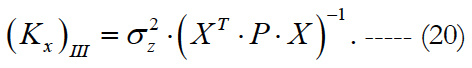
3. Without parameterization (the optimum filtration of measurements). The a priori correlation matrix of interfering parameters is used for "weighting" the measurements without state vector extension. The effect of interfering parameters is taken into account by their association with measurement errors, and then the maximum likelihood technique is applied. In this case, the required estimate is determined by formulas (7) and (8), and its correlation matrix is expressed as follows:
Now we pass to transforming expression (20) into the form convenient for comparison with estimates (12) and (17). In this case, it is convenient to use the well-known lemma [12] on the inversion of matrices:
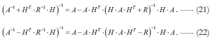
We use formula (21) to transform the weighting matrix expression (8) to the more convenient form for comparison. We get:
We denote the expression in brackets in the right-hand side as R
Then substitution of (23) into (20) leads to the following expression:
We perform inversion of this matrix using formula (22).

We denote the expression in square brackets in (26) as C and take into account (24). We get:
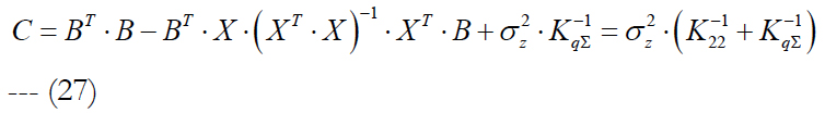
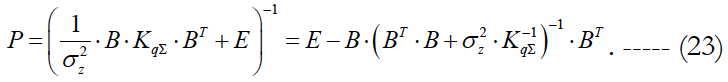
Finally, formula (20) can be written as:

We compare this estimate with similar estimates (12) and (17) for the first and second approaches to evaluating the state vector. With accounting for formula (28), we write down the expressions for relevant differences:
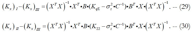
The relation of these differences depends on the relation of differences in brackets. For their further analysis, we use formulas (27) and (21). We get:
These formulas have beautiful symmetrical appearance. The values of differences depend only on two matrices KqΣ and K22. The first of them characterizes the noise level, and the second one – the information capabilities of updating them based on available measurements. In the presence of noises (KqΣ ≠ 0) the differences represent positively defined matrices. Substituting these formulas into (29) and (30), we get the important expressions:
From them we obtain the following conclusions.
Optimal filtration of measurements increases accuracy of estimates as compared to LST without regard to interfering parameters.
Optimal filtration of measurements increases accuracy of estimates as compared to LST with regard to interfering parameters (parameterization).
Thus, as a result of a alysis, the comparative relationships were established between the errors of state vector estimates with using the considered methods (approaches). The analysis results are presented in Figure 2.

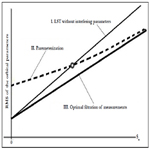
Figure 2. Dependence of errors on the applied approach and the signal-to-noise ratio.
It is seen from figure’s data that, for any level of disturbances, the best accuracy is achieved with applying the optimal measurement filtering technique. The expediency of LST application without or with state vector extension depends on the level of disturbances. There exists some level of small disturbances, at which it is more expedient to apply LST without state vector extension. However, even in this case the errors are greater, than in the case of using the optimal filtration of measurements (the nonparametric approach). This conclusion agrees with results published in papers [7, 9, 10]. The application of a nonparametric approach is a perspective direction for increasing the orbit determination and prediction accuracy. In the course of its application, it is necessary to take into account the statistical characteristics of random disturbances.
Conclusion
The application of joint measurements processing in updating satellite orbits faces the necessity of correct accounting for random perturbations. In the early 70-ies it was suggested to improve the least square technique based on accounting for random perturbations in "weighing" the measurements. This improvement was called the method for Optimal Filtration of Measurement (OFM).
The comparison of the accuracy of estimates, obtained with using the LST (with extension and without extension of the state vector), as well as the OFM method, was performed. It was shown that, in the presence of perturbations, the application of the OFM method provides the best accuracy.
References
- Ivanov NM, Lysenko LN. Ballistics and navigation of spacecraft. M. Publishing house MVTU them. Bauman;2016. 524 p.
- David A. Vallado Fundamentals of Astrodynamics and Applications. 4th ed. Microcosm Press, Cluwer Academic Publishing;2013.966 p.
- Nazarenko AI, Markova LG. Technique for Correction and Prediction of Orbits With Taking Into Account the Motion Model Errors. Articles Applied tasks of Space Ballistics,«NAUKA», Moscow;1973.
- Nazarenko AI. Determination and prediction of orbits with due account of disturbances as a'color' noise. Space Flight Mechanics Meeting. Monterey, CA;1998. 98-191.
- Nazarenko AI, Yurasov VS, Alfriend KT, Cefola PJ. Optimal measurement filtering and motion prediction taking into account the atmospheric perturbations. InAAS/AIAA Astrodynamics Specialist Conference; 2007. 07-363.
- Nazarenko AI. Accuracy of determination and prediction orbits in LEO. In Estimation Errors Depending on Accuracy and Amount of Measurements, Seventh US/Russian Space Surveillance Workshop, Monterey; 2007.
- Nazarenko AI. Increasing the accuracy of orbit forecasting on the basis of improvement of statistical methods for processing measurements. In Fifth European Conference on Space Debris;2009. 672.
- Nazarenko AI. Errors of forecasting of satellite motion in the Earth gravity field. Institute of cosmic research; 2010. 225 p.
- Nazarenko AI. Application of the technique of optimum filtration of measurements for updating and forecasting the spacecraft orbits. Vestnik, Science-Technical Journal. S.A. Lavochkin Science-Production Association, Federal State Enterprise,No. 2; 2012.
- Nazarenko AI. How can we increase the accuracy of determination of spacecraft ׳ s lifetime?. Acta Astronautica; 2015 Nov 1. 116 :229-36.
- A.I. Nazarenko. Some questions of optimization processing orbital measurements of artificial Earth satellites. Space research;1968. 6:674- 683.
- Robert C.K. Lee. Optimal estimation, identification and control. Research monograph No 28, The M.I.T. press, Cambridge, Massachusetts; 1964. 176 p.