Lamb Waves for Detection of Delamination in Composite Plates

Keywords

Delamination; Lamb Waves; C-Scan; Wavelet; Tomography; Carbon-Composite.

Introduction

In recent years there has been a high incorporation of composite material in aerospace industry due to their unique strength to weight ratio and corrosion endurance. However, due to the composite layer nature of such materials, they are susceptible to production and usage strength deterioration that reduce material strength. This tendency results in an increasing need for soundness monitoring the structure and detects structure damages known as delamination. Such damage types are hard to locate since the material is highly ununiformed and the delamination is not visible. There are some methods developed in order to locate such structural damage but each has its own limitations and difficulties. There is a need for method that can identify delamination as a standalone and integrated part of an array of tests in order to create a highly trusted and reliable detection system. Delamination can be caused by either a fault in production, a small air bubble that is trapped in between the layers, or developed during operation. The epoxy resin is subject to stress or impact and the layers begin to separate. Unlike other methods that require the disassembly of parts in order to examine them, the suggested method in this paper can be used to scan a complete panel while it is still assembled on the airplane\UAV.

Several other methods for locating delamination exist, each with its own strength and weaknesses, such as the Tapping inspection tapping on the composite structure with a metal hammer and listening for a change in sound as different places are impacted. The Tapping technique is limited in scope as small defects are difficult to detect. Detectability of defects is inversely proportional to surface skin thickness. Ultrasonic Pulse-Echo (PE) inspection is the most commonly used method for inspection of composite materials. It is based on one piezoelectric (PZT) probe, which transmits a relatively high frequency sound wave through a couplant liquid to the tested object. As the acoustic impedance in the structure changes, whether it is from a defect or a boundary, it reflects the wave back to the probe, which receives the signals and displays an amplitude – time presentation (A-Scan) of the received signals. This method can determine the depth and size of the delamination.

Through Transmission Ultrasonic (T.T.U.) is similar to the PE method in high frequency transmission, yet a different PZT probe is the signal receiver. This method cannot determine the depth of the delamination, yet it has a relatively reliable outcome for defect detection. Ultrasonic Phased Array (PA) uses a special highfrequency inspection technique that makes use of transducers consisting of multiple ultrasonic elements that can each be driven independently. It produces a scanning image of the tested area (C- Scan) and can swiftly determine the defect shape and depth as well as the porosity level of the material [16]. Air Coupled Ultrasonic (ACU) utilizes a non-contact low-frequency and high penetration inspection, which is similar to the T.T.U. principal. It can present the shape of the defect in a low resolution. However, it allows inspection of Foam structures, which are not suitable for water coupling detection, as well as allowing a rapid inspection of large structures. Resonance inspection applies a low-frequency resonance method by using special narrow bandwidth ultrasonic contact probes. Inspections are performed by monitoring the electrical impedance of the transducer at a signal frequency, the working frequency. A transducer’s electrical impedance depends on the mechanical load on the surface [17]. The Pitch-Catch or Sondicator method uses a pair of transducers displaced from each other by fixed distance. A single low ultrasonic frequency is transmitted into the part by one transducer.

A second transducer in the same probe receives the returned signal. Radiography is the deployment of beams of ionizing radiation to the non-destructive testing of structures. The basic principle is that flaws that have differing radiation absorption properties can be discriminated in the image formed by the beam transmitted through the part. It is mostly applicable for splice bonding inspection [18]. While these methods usually produce good results, they are sometimes expensive or limited in their scan time and result. Lamb Waves are widely used in different approaches and configuration [2]. Uses a square PZT formation and a computer simulation in order to train an artificial neural network [8]. Uses a fiber-optic sensor in order to detect and analyze the dispersive curves of different propagation modes [11]. Uses mode velocity analysis in a circle sensor formation that requires prior knowledge of the group velocity-propagation profile in order to image a discontinuity in the carbon fiber reinforced plastic(CFRP) [3, 11]. both present a 2-sensor configuration based on a stimulating beam and analyzing the returned echo of the signal while depending on Finite element method (FEM) simulations [6, 12]. produce a tomography scan by using 2 sensors that directly analyze the signal rather than investigate the signal echo and combining the data to create a C-Scan. The presented configuration uses a circle configuration and wavelet-based signal analysis in order to harvest data following machine learning methods to decide if the signal has been effected by a delamination or not and combining several sensor decisions in order to create more reliable results and producing a C-Scan using natural neighbor interpolation [7].

Lamb Waves

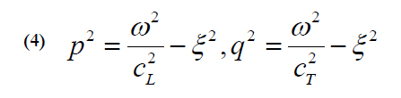
Lamb Wave theory refers to the movement of mechanical waves in a thin free plate. The waves move on the upper and lower parts of the free plate. This theory is devolved and documented in a number of textbooks and articles [14, 15]. The following section will introduce the basic concept for the analysis of such waves. The wave equations are:

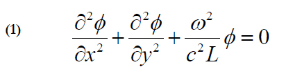
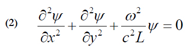
Where Ø and ψ are two potential functions c²L = (λ +2μ)/ρ and c²T = μ/ρ are the pressure and shear wave speeds λ and μ are the Lamb constants, and ρ is the density. It is assumed that the time dependence is harmonic in the form of e-iwt. Therefore, the solution of equations 1 and 2 is given by equations 3 and 4.

Where ξ= ω/c is the wave number and:

The four integrations A1, A2, B1, B2 constants will be found by the boundary conditions. Using the relation between them results in equations 5, 6 and 7:

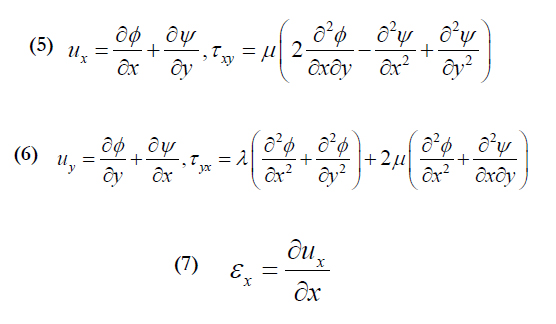
From that, we obtain:

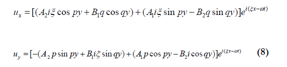
There exist two forms of motion symmetric and anti-symmetric that corresponds to the two terms in equation 8. In order to calculate free wave motion the homogenous solution need to be derived by applying the stress-free boundary condition at the surfaces ( y = ± d, where d is half the thickness of the plate) the compact form known as the Rayleigh-Lamb equation can beobtained by equation 9.

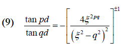
Where +1 describes the symmetric (S) mode and – 1 the antisymmetric mode (A).

There is an inherent relationship between these equations, in particular the angular frequency ω and the wave number along with other coefficients that yields different Lamb mode shapes designated as S0,S1,S2… and A0,A1,A2 … corresponding to symmetric and anti-symmetric accordingly. Due to this relationship, the wave speed will change according to the excitation frequency and produces wave dispersion. For every plate thickness and frequency the predicted wave speed will change, this model is for isotropic infinite plates. While in realty the carbon-based composites are neither isotropic nor infinite and this model gives a close approximation and understanding for the behavior and interaction of waves in a plate and with delamination.

×

Figure 1

Close

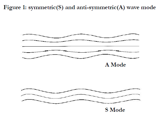
Figure 1: symmetric(S) and anti-symmetric(A) wave mode

Data Collection

A setup consists of an AEwin Mistras system with an 8 channel, 16 bits, 400 kHz Bandwidth, PCI Bus card capable of recording simultaneously data from 8 PZT sensors is used to gather Lamb Wave signals for the purposed data. Creating an Acoustic Emission (AE) signal was implemented using the Arbitrary Waveform Generator Board PCI-Based, 14-bit, 100 M sample/sec, +/- 150V output, 700 kHz Bandwidth with manual and WaveGen software. 3 Carbon Fiber Woven Fabric, Epoxy Pre-impregnated reinforced polymers (CRFP) panels where used in this study. The reference panel’s dimensions were 593 x 590 mm, 596 x 588 mm, the delamination containing panel is 593 x 590 mm with delamination of size 35 x 35 mm and all have 12 layers of carbon fiber in an alternating 0/90,-45/45 orientation. The system includes eight 180 kHz main frequency 14 mm circular PZT sensors amplified by a 43dB pre-amplifier. The sensors are denoted S1-S8, and are placed in a circle configuration with a radios of 10 cm on the CRFP panels. Excitation of vibrations on the panel is implemented using each of the PZT sensors with a single-pulse sine wave of 180 kHz for a duration of 0.05 milliseconds created by 10 repeated cycles, as shown in Figure 2.

×

Figure 2

Close

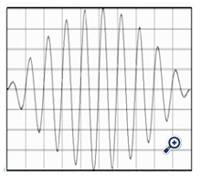
Figure 2: waveform of the signal transmitted by the transmitter sensor

The setup includes of 8 PZT sensors placed on a composite panel in a circle with radius of 10 cm. A sensor “image” is built by using one sensor as a transmitter, transmitting a fixed signal and the other 7 sensors as receivers, recording the ultrasonic signal transmitted. This process is repeated 8 times for each of the sensors in the circle. The result is one “image” of 7 recorded signals from each sensor associated with the transmitter location. Figure 3 illustrates sensor positioning on the panel.

Using the above configuration, several “images” or recorded data where taken. The “image” is the combination of all pairs of transmitter-receiver possible signals recorded in a circle in a given location. The images are recorded in different locations containing both a delamination and a reference’s non-delaminated area of the panel. The location of delamination in the panel and the verification that other areas of the panels are undamaged are verified by using the ACU method as Figure 4 shows. Creating a data set of 9 images taken from several panels, 6 images used only for training and 3 for testing, due to difficulty in obtaining panels containing delamination, the same panel was used several times in different locations of the delamination with respect to the sensors circle and several for every location on the panels - 3 images were taken every time.

×

Figure 3

Close

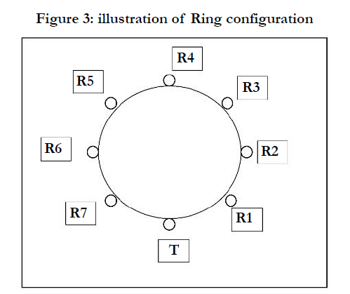
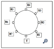
Figure 3: illustration of Ring configuration

Excitation of waves

The proposed model operates by analyzing the changes in the recorded signal of a known transmitted signal. The transmitted signal is fixed and produced by a PZT transmitter sensor with a known form, energy and frequency; the form is of a sinus wave with a frequency of 180 kHz 10-cycle pulse. We arrived at these defining parameters by trial and error. Different parameters where tested on a 2-sensor configuration and the most responsive was selected. These parameters are not necessarily optimal for all kinds of delaminations but responsive enough for our needs. Further research is needed. The wave function can be seen in the figure 2.

Signal Processing and Pattern Recognition

Wavelet Transform

Wavelet transform as introduced by [19] Meyer, enables transforming the recorded acoustic signal into a frequency-time dependence space unlike a Fourier transform that only displays the main frequencies that the signal is constructed by. The wavelet transform enables a view of both frequencies and the time in which it occurs. Since analyzing propagating waves is affected both in velocity and in frequency, it is an important tool for analyzing the signals. Wavelet transform has been reviewed by many papers [20, 21], this paper will present the very basics of the transform.

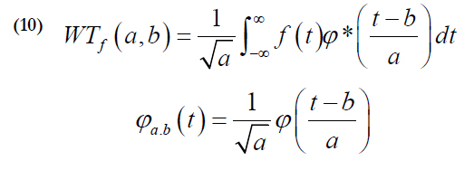
Where a>0 and * denotes a complex conjunction a in the scale of the function in the Wavelet Transform (WT) that corresponds to frequency a and the b variable is a shift of the function, which is a shifting and scaling of variables of the original wavelet φ(t).

In WT, there is a relation between the scale factors 'a' to the frequency of the signal, higher scale’s correlate with a higher frequency. One can view the process as a sliding window for both parameters a and b where changing. a yields a different frequency correlation and changing b yields the correlation of the function of a - a specific part of the input function (or recorded signal) f(t).

SVM

SVMs are the result of extensive work in computational learning theory. Their high accuracy is drawn from their ability to use a relatively small number of training examples and still find a separation that yields good results by maximizing the gap between the hyper planes and training examples. Also, it has a proven ability for separating data that cannot be linearly separated, by mapping it into a new higher dimensional space using a kernel function. In the higher dimensional space, the data can be separated. Computationally, the SVM algorithm finds the best location of the decision plane by solving an optimization problem. The SVM finds a hyper-plane that has the maximum margin from both classes of data. Formally let us suppose that we want to classify two classes as in our case, if a phenomena has happed or not. Given a training data of n data points, each point is defined by equation 11.

Where the values of y correspond to whether the data is in class 1 or 2, xi is the m-dimensional real vector of the data point. The goal is to find a hyper-plane that maximizes the margin of the division between all points of yi=1 and yi= −1. The optimal dividing hyper-plane can be written as (equation 12).

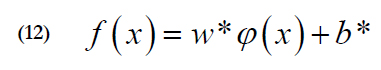
It is defined by the optimal weight vector w* Є Rm and the bias b*Є R, where φ(x) is a kernel function that first mapped a data point from m-dimensional space into a higher dimensional feature space. These optimal w* , b* are the ones that minimizes the cost function that expresses a combination of two criteria, margin maximization and error minimization. This function is also subject to constraints and can be reformulated in a form that Lagrange multipliers can be found by using the dual optimization of the following equations 13, 14 and 15.

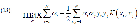
Under constraints:

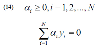
Where α=[α1, α2,..., αN] is the Lagrange multiplier vector. The final result, following the maximization problem, is a function of the original data feature space dimension m

Where K (xi, x) is a kernel function; b*,α*i are the optimal bias and weight. V is a subset of the indices {1, 2 …, N} which correspond to non-zero Lagrange multipliers, which indices the support vectors, from a geometrical point of view.

SVM Training

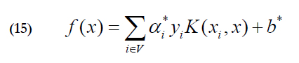
As previously explained (Section 2), the dataset for training consist of 6 images, 3 of reference panels and 3 of damaged panels containing delaminations. Since the image is captured in a circle configuration, each image is compiled from 7 input acoustic recording signals for each of the 8 transmitting sensors. Hence, there are 7 pairs that correspond to 4 different distances as shown in Figure 4. The 6 images resulted in a 1008 rows. In order to simplify.

×

Figure 4

Close

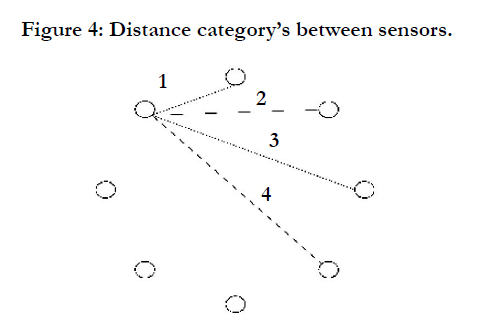
Figure 4: Distance category’s between sensors.

Figure 5; a. an example of recorded signal b. the signal wavelet transform c. mean side look of the wavelet transform Facilitate the SVM training the data, they were subdivided into 4 categories based on the distance between transmitter and receiver. For each category, a separated SVM was trained. We used the wavelet transform to create a measurement of discriminative properties from the signal. First, the input signal was transformed using the Moral function in scales of 1 to 20. Following that a mean function was implemented, which reduced the 3D wavelet transform into 2D space, as seen in Figure 5c.

×

Figure 5

Close

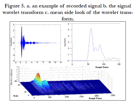
Figure 5. a. an example of recorded signal b. the signal wavelet transform c. mean side look of the wavelet transform.

The input signals were classified into 4 categories depending on the length between transmitter and receiver. Each length, noted 1-4, was trained separately but used the same feature as a basis for classification, as shown in Figure 4. In the first stage, a wavelet transform was applied to all recorded signals, as illustrated in Figure 5. The wavelet function used was the Morel function with a scale range of 1-20. In the second stage, the wavelet transformed signals were mean-averaged across the scale axes resulting in a two-dimensional plot amplitude/time. After further examination of this plot illustrated in Figure 6 it is clear that while the signal that passed through a plate showed the same wavelet characteristics, even in different orientation; i.e., all signals of length 4 that were recorded showed the same wavelet profile independent of their orientation on the plate. The wavelet profile of a signal that has gone through a delamination is usually altered, mainly in the distance between the first high peak and the second high peak corresponding to different wave modes S0 and A0 as Figure 6 shows.

×

Figure 6

Close

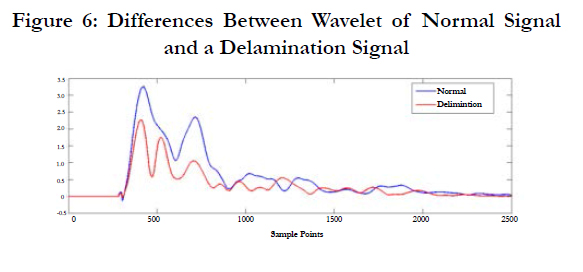
Figure 6: Differences Between Wavelet of Normal Signal and a Delamination Signal

Following this observation, a distance function was established between the peaks as Figure 7 shows. Distance measurement of the wavelet profile was the main classifier the SVMs were trained on.

×

Figure 7

Close

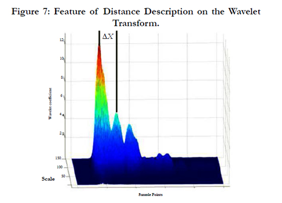
Figure 7: Feature of Distance Description on the Wavelet Transform.

Validation of the location of delaminations and the integrity of the plates was verified by an independent Air-scan Saar Radar [13]. As seen in Figure 8, Figure 9 illustrates a side view of the delamination.

×

Figure 8

Close

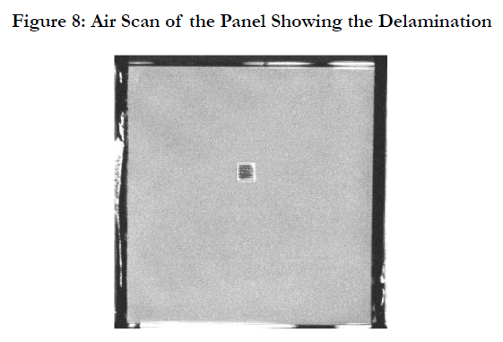
Figure 8: Air Scan of the Panel Showing the Delamination

×

Figure 9

Close

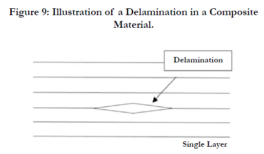
Figure 9: Illustration of a Delamination in a Composite Material.

This configuration of the SVM yields good results in detecting whether a signal is affected by a delamination and can be easily adopted for different types of plates.

Image Reconstruction

Natural Neighbor Interpolation

As introduced by Sibon, natural-neighbor interpolation enables completing a scatter map of data into a more dense/continuous map by sampling values from a neighbor’s point taking into account the density and distance between data. Using this method yields better and smoother results when reconstructing the points into a map. Natural neighbor-interpolation works as follows, for a set of points denoted as X = [x1,....,xn] where xi are points each having a corresponding value v1,...vn. n order to add a new point xp with an unknown value vp that we wish to interpolate, first a Voronoi diagram of our data points X is constructed denoted as D. Than a new Voronoi diagram is constructed including the new point X'={X U xp} denoted as, Dp. Figure 10 shows the difference between such diagrams. For each of the diagrams, Dp ,D, we mark the volume and area of every cell corresponding to a point with Cx for points from D and Cx DP for points from Dp.

Now for each neighboring points of the new point xp; i.e., the points xp share a border with, we can calculate approximate weight by the relation between of the volume of a cell in the old diagram D and the new diagram Dp

The calculated estimated value of point xp based on its neighbors is given by the values of the points weighted by the proportion of crossing volume.

×

Figure 10

Close

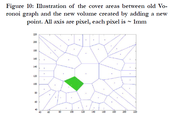
Figure 10: Illustration of the cover areas between old Voronoi graph and the new volume created by adding a new point. All axis are pixel, each pixel is ~ 1mm.

Tomography

Following this concept, we take the recorded “image” from the sensors and construct a map. The transmitter sensor is denoted T while the receiving sensors are denoted R1−7 as illustrated in Figure 3.

By implementing the decision algorithm upon the signal recorded by sensor Ri that can identify whether or not a delamination interrupted the propagating Lamb Waves created by sensor T, a tomography map can be synthesized. Figure 11a illustrates the connection between each sensor pair. It can be seen that there are intersecting points in the graph that are created from the crossing of 2 sensor pairs or more at the same geometrical point. These points are shown in Figure 11b, the intersection points are of high value to the tomography reconstruction due to its reduction of individual decision errors. By considering multiple classifications of the signal that were propagated, it projects a delaminationcontaining area. The certainty of that geometric point as a delamination containing area is greater than having to rely on a single classification of the signal.

×

Figure 11

Close

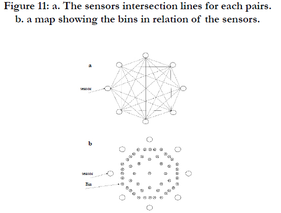
Figure 11: a. The sensors intersection lines for each pairs. b. a map showing the bins in relation of the sensors.

A Bin is created for each geometric crossing point of an edge. For an 8-sensor circle graph there are 48 relevant bins noted as BINk. Every bin BINk is associated to a pair Ti − Rj if the line between the sensors includes the geometric point matching BINk, as shown in Figure 2b.

For every pair Ti − Rj that is classified as having passed through a delamination all Bin on the line associated with the pair, one is added, resulting in a map illustrating the number of classifications per bin, as illustrated in Figure 11b. By following this scheme, the location of a delamination relative to the sensors position is detected, with a higher probability than simply using 2 sensors.

Since the bins are not continuous and provide only a low resolution image of the delamination, a natural interpolation function is employed for the bins as described in Section 4.1, resulting in a smooth image describing areas of high probability for containing a delamination. This scheme is as strong a classifier as can be relied upon. By using the amplification of considering several classifications, the error rate is decreased.

Further research is needed to create a more accurate classifier that yields true results with higher probability, or a non-binary classifier that produces the probability that the signal is passing through a delamination.

Results

There are two ways to view the results. One way is to measure the individual signal classification of our classifier by considering the classifier decision as compared to a known delamination location. While the other is by examining the C-scan produced as the final result in comparison with the delamination location. Since the original classification on the training data had an inherent uncertainty whether or not the phenomena would be caused by the delamination, the training classification was concluded simply by the fact that the signal has passed through the vicinity of a known delamination location. Also, since the final objective is the creation of a C-Scan map, and the point has some multiplicity in detection it is far more desirable to create a decision algorithm that produces false negative rather than false positive.

Table 1 illustrates the prediction accuracy of the decision algorithm developed on recorded signals separated by length.

×

Table 1

Close

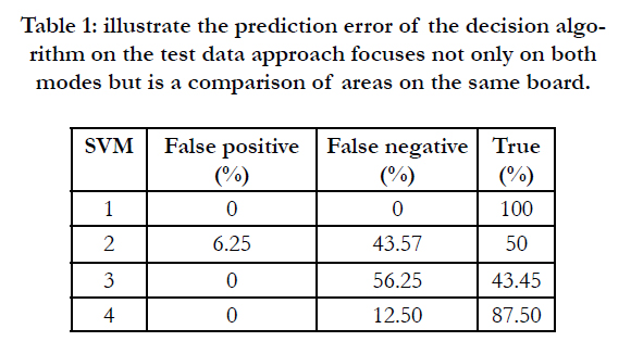
Table 1: illustrate the prediction error of the decision algorithm on the test data approach focuses not only on both modes but is a comparison of areas on the same board.

This Sensor length of 1 and 2 are less relevant since there is small training data containing delamination that affect length 1 and 2, also the key features manifest better at greater distances.

Figure 12 illustrate the C-Scan of the test samples. The test data is 2 images of the same delamination in different position in relation to the sensors. And a reference image without delamination.

×

Figure 12

Close

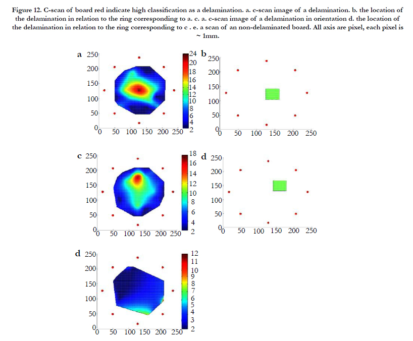
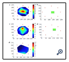
Figure 12. C-scan of board red indicate high classification as a delamination. a. c-scan image of a delamination. b. the location of the delamination in relation to the ring corresponding to a. c. a. c-scan image of a delamination in orientation d. the location of the delamination in relation to the ring corresponding to c . e. a scan of an non-delaminated board. All axis are pixel, each pixel is ~ 1mm.

Discussion and Conclusion
This paper presents a hands-on approach for detecting delamination in a CFRP panel. This approach can be easily calibrated for different types of panels. Using a few reference scans of the panel, the descriptor can be calibrated for a new mean-average allowing for a highly versatile approach for detecting delaminations. [2] Suggest a neural network approach that requires access to a simulation of a panel’s delamination signals or a lot of real measured data to train the network. Therefore, training for new panels is a complicated task [12]. Uses arrival time and frequency change to detect discontinuity on the surface using only S0 mode. This approach is practical but is not suitable for detection of delamination. Our results in a powerful and versatile tool that detects changes in expected values based on global data.

Future work can be done to locate a delamination based not on SVM classification but on changes in values of several descriptors with regard to the entire panel’s recorded values, where an anomaly in such values is associated with the existence of delamination. To conclude, this study presents a configuration for the detection of a delamination in carbon-based composite okay plate like structure and creation of the C-Scan tomography map. Although this study was limited in hardware resulting in poor resolution and the creation of a C-Scan that is limited to the sensor circle area, the model can be easily developed further in order to create a high-density full-plate C-Scan by combining scanned data from multiple locations on the plate. Also, by adding other feature extraction methods, the accuracy of the decision algorithm can be increased and the C-Scan produced can have greater detail. The method developed presents a solid foundation in the detection of delamination by using analytical algorithms that analyzes alterations in the recorded signal itself and translating the recorded signal into a C-Scan map.

Acknowledgment

The authors thank the NDT/E Laboratory at the Israel Aircraft Industry for funding this study and providing the required equipment for the presented experiments.

References

- Valdés SH, Dıaz CS (2002) Real-time nondestructive evaluation of fiber composite laminates using low-frequency Lamb waves. J Acoust Soc Am. 111(5): 2026-2033.
- Su Z, Lin Y (2004) Lamb wave-based quantitative identification of delamination in CF/EP composite structures using artificial neural algorithm. Composite Structures. 66(1): 627-637.
- Hu N, Li J, Cai Y, Yan C, Zhang Y, et al., (2012) Locating delamination in composite laminated beams using the A0 lamb mode. Mechanics of Advanced Materials and Structures. 19(6): 431-440.
- Giurgiutiu V (2005) Tuned Lamb wave excitation and detection with piezoelectric wafer active sensors for structural health monitoring. Journal of intelligent material systems and structures. 16(4): 291-305.
- Boissonnat JD, Frédéric C (2000) Smooth surface reconstruction via natural neighbour interpolation of distance functions. Proceedings of the sixteenth annual symposium on Computational geometry. ACM. 7: 223-232.
- Jansen DP, Hutchins DA, Mottram JT (1994) Lamb wave tomography of advanced composite laminates containing damage. Ultrasonics. 32(2): 83- 90.
- Sibson R (1980) A vector identity for the Dirichlet tessellation. Mathematical Proceedings of the Cambridge Philosophical Society. 87(1): 151-155.
- Li F, Murayama H, Kageyama K, Shirai T (2009) Guided wave and damage detection in composite laminates using different fiber optic sensors. Sensors. 9(5): 4005-4021.
- Park SW (2006) Discrete sibson interpolation. Visualization and Computer Graphics in IEEE Transactions. 12(2): 243-253.
- Boissonnat JD, Frédéric C (2001) Natural neighbor coordinates of points on a surface. Computational Geometry. 19(2): 155-173.
- Hu N, Shimomukai T, Yan CW, Fukunaga H (2008) Identification of delamination position in cross-ply laminated composite beams using S 0 Lamb mode. Composites Science and Technolog. 68(6): 1548-1554.
- Liu Z, Yu F, Wei R, Wu B (2013) Image fusion based on single- frequency guided wave mode signals for structural health monitoring in composite plates. Mater Eval. 71: 1434-1443.
- Hsu DK, Komareddy V, Barnard DJ, Peters JJ, Dayal V (2004) Aerospace NDT using piezoceramic air-coupled transducers. Proceedings of the 16th WCNDT.
- Viktorov IA (1967) Rayleigh and Lamb Waves: Physical Theory and Applications. Plenum Press, New York.
- Achenbach JD (1984) Wave Propagation in Elastic Solids. (1st edn), Elsevier, New York.16: 1-440.
- Sol U, Kleinman M, (2012) Ultrasonic Inspection of Composite Laminate and Bonded Structure. Israel Aerospace Industry Documentation, PS812050.
- Sol U, Kleinman M, (2012) Resonance Inspection Using Bondascope 2100. Israel Aerospace Industry Documentation, PS812070.
- Leibovitz H, Green AK (2012) Radiographic Non-Destructive Inspection- General. Israel Aerospace Industry Documentation, PS811000.
- Meyer Yves, David H Salinger (1995) Wavelets and operators, press, Cambridge university, England. 1.
- Chui, Charles K (Ed.) (2014) An introduction to wavelets. Academic press. 1.
- Akansu Ali N, Richard A Haddad (2001) Multiresolution signal decomposition: transforms, subbands, and wavelets. Academic Press.