Piecewise Hazard Modeling for Under-Five Child Mortality
Saroj RK1*, KN Murthy2, Kumar M3
1 Research Fellow, Analysis Unit, Centre for Infectious Disease Research in Zambia, Lusaka, Zambia.
2 Associate Professor,Institute of Medical Sciences, Banaras Hindu University, Varanasi, India.
3 Assistant ProfessorStatistics Section, MMV, Banaras Hindu University, Varanasi, India.
*Corresponding Author
Rakesh Kumar Saroj,
Research Fellow, Analysis Unit, Centre for Infectious Disease Research in Zambia, Lusaka, Zambia.
E-mail: rakesh.saroj@bhu.ac.in
Received: May 11, 2019;Accepted: November 25, 2019;Published: November 27, 2019
Citation: Saroj RK, KN Murthy, Kumar M. Piecewise Hazard Modeling for Under-Five Child Mortality Int J Translation Community Dis. 2019;7(1):104-111. doi : dx.doi.org/10.19070/2333-8385-1900017
Copyright: Saroj RK© 2018. This is an open-access article distributed under the terms of the Creative Commons Attribution License, which permits unrestricted use, distribution and reproduction in any medium, provided the original author and source are credited.
Abstract
Objective: The application of piecewise hazard model in mortality data becomes more useful over classical survival methods. This method is used to find the number of location of cut points and estimate the hazard model. The piecewise hazard model is fitted on National family health survey (NFHS IV) from different variables like socio demographic, biological and proximate co-factors.
Methods: The various methods are used to apply on mortality data. Exponential hazard model, Weibull hazard model and piecewise constant hazard model are illustrated on mortality data. Cox regression analysis is also performed to find the significant role of co-factors. Free R software is used analysis of mortality data.
Results: It is found that women’s age in years, total children ever born, present breastfeeding, smoking, size of child, delivery by caesarean section, ANC visits, and birth orders are important factors and six month time interval is very crucial for child till completing the five year of the age.
Conclusion: Piecewise hazard model is found very important for the under-five child mortality, through the various times cut point. The Piecewise hazard model can be useful for clinicians, researchers and public health experts. Time is very important factor for reducing the child mortality.
2.Introduction
2.1 The relationship between survivor function and hazard function
2.2 Piecewise-constant hazard model
3.Material and Methods
4.Result
5.Conclusions
6.References
Keywords
Under-Five Childrenmortality; Piecewise Hazard; Survival Analysis; NFHS-IV, R software.
Introduction
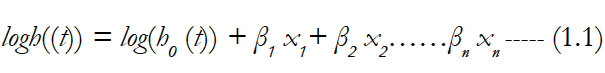
The survival analysis is a technique to quantify the patient's survival that after treatment in a specifics infection. Survival and reliability is defined as reliability use for machine working period or machine solid in period, while survival analysis use in life the survival status of patients. In the survival techniques; measure the survivor function, or the hazard function. The hazard is the momentary occasion (demise) rate at a specific time point t. In survival techniques doesn't expect the hazard is consistent after some time. The aggregate hazard is the cumulative hazard experienced up to time t. The survival function is likelihood an individual survives up to and including time t. The likelihood the occasion (e.g., demise) hasn't happened yet. The Kaplan-Meier curve appraises the survival curve of patients who representing the proportion of patients who survived over time [1]. The Cox PH regression technique is reasonable for survey the impact of both categorical and continuous variables, and could be model the effect of multiple variables at once [2]. The Cox PH regression models characteristic log of the risk at time t, signified by h (t), as a function of the baseline hazard (h0(t)) and a few indicator factors x1,x2,… … xn. The model is.
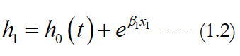
Take the exponentiation both sides of the equation, and limit the right hand side to just a single categorical exposure variable (x1) with two groups (x1 = 1 for exposed and x1 = 0 for unexposed), the equation becomes:
After solve the equation estimate the hazard ratio, comparing the exposed to the unexposed individuals at time t by given formula:
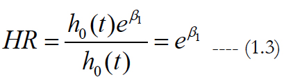
The eβ1 is the hazard ratio and other constant over time t. The β is the regression co-efficient that estimate from model and represent the log(Hazard Ratio) for each unit increase in the corresponding predictor variable.
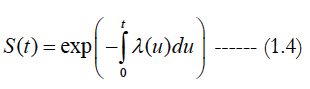
Let G (t) = log S(t) Then the derivative of G (t) is written as:
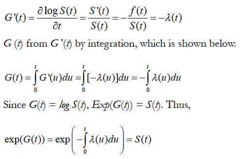
Thus, the relationship between the survivor function and the hazard function is given by:
Let x be the row vector of explanatory variables, and β be the corresponding column vector of coefficients. The model hazard function λ(t, x, β) as,
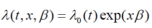
λ0(t) is called the baseline hazard. There are several choices for the baseline hazard models are exponential hazard model, Weibull hazard model and Piecewise-constant hazard model.
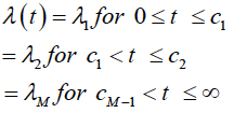
An essential expansion of the exponential model is known as piece-wise exponential model or piecewise- constant hazard model. This model originates from an appropriation whose hazard rate is a step function. It will be moved relatively relying upon the group parameters. This model is most adaptable and easy yet great group of models. In this model, need to fragment the survival into a numerous pieces. In this model accept that inside each fragment, the hazard is constant but between segments, hazard could be different. The hazard function can be written as:
Assume the segment the survival into three pieces, 0 ~10, 11~20, 21~∞. Give B1 a chance to be the fake variable that takes 1 if the recorded survival is in the primary section. B2 is the fake variable that takes 1 if the recorded survival is in section 2. B3 is the sham for those whose recoded survival is in fragment 3. To measure the piecewise-constant hazard model. Let us divide the fragment in the accompanying way:
Segment 1: 0~5 years
Segment 2: 6~10 years
:
Segment 5: 21~25 years
Segment 6: 26 years or greater
In this study assessing the basic hazard function with likely time change points. It will demonstrate the survival pattern of the patients and which time points is more demise or more censor. Assessing the survival trend for entire population will give better comprehension of how changing treatment, patients monitoring, health facilities of patients, and public health services, affect the population survival analysis. Likewise, find the individual understanding the hazard function including how and when changes in the risk for death happen, considers an actual existence way perception.
Past researches have proposed strategies for finding a solitary change point in a piecewise consistent hazard function [3]. None but less, in the clinical research and expanding survival rates of patients accept there might be a few situations where a model with at least two change points is more proper [4]. This technique is used for change points in prostate cancer death rates [5]. Built up a piecewise-exponential methodology where Poisson regression model parameters were assessed from pseudo-probability and the comparing differences were determined by Taylor linearization strategies [6]. The study is demonstrated the estimation of a change point in a hazard function dependent on censored data [7]. Another study shows the piecewise constant hazard model to evaluate the mortality inferable from some normal risk factors [8]. In a research article, it is proposed another strategy to naturally locate the suitable number and area of the cuts utilized in this model [9]. Another study has done to find the survival status of under-five child mortality in Uttar Pradesh [10]. Proposed this model under-five child survival status through NFHS-IV information of Uttar Pradesh and taken the various time points for finding the adjustments in the constant hazard function in this study.
Material and Methods
Secondary data has been taken from NFHS-IV of Uttar Pradesh under-five children data sets. For analysis, the age of the children in months is ascertained as pursues: age = V008 – B3, where V008 is the century month code (CMC) of the date of meeting, and B3 is the CMC for date of birth of the kid. The variables affecting under-five child survival from the data set is chosen dependent on the paper by Mosley [11]. These components were sorted into the accompanying four classifications; Social demographic and social economic, environmental and proximate or biological factors but in this paper used the analysis based on three social demographic and social economic, proximate and biological factors only. First calculated the important factors who play the important role in survival of the child mortality through Cox-regression analysis after that those important factors used in the piecewise constant hazard analysis. All the analysis done through MS-Excel and R 3.2.
Result
The Table.1 shows that survival status of under-five year children. In this table shows that total 93% cases censored as per data because child death is considered event under study. Total survival time of children is 59 months (Figure 1) and plot shows the survival probability and censor cases report of children, where + symbol is the censor in the graph. In the table 1.1 shows the socio-economic and demographic factors to play important role in child survival status through Cox-regression. It is found that educational level, women's age in years and religion play significant role in the child survival status. In the Table 1.2 calculated the environment factors to play important role in child survival status and none variable found significant role in the child survival status.
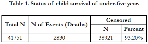

Table 1. Status of child survival of under-five year.
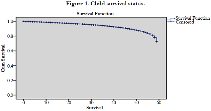
Figure 1. Child survival status.
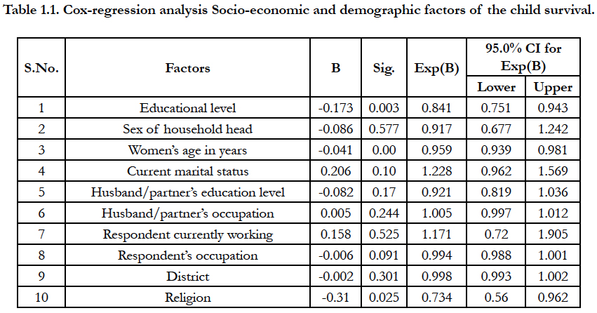
Table 1.1. Cox-regression analysis Socio-economic and demographic factors of the child survival.
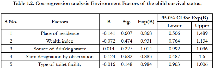
Table 1.2. Cox-regression analysis Environment Factors of the child survival status.
In the table 1.3 It is calculated the proximate and biological factor to play important role in children survival status and find that variable like children ever born, births in last five years, number of living children, currently breastfeeding, smokes cigarettes, desire for more children, weight of child at birth, delivery by caesarean section, ANC visits and birth order play significant role in the survival status of children. Cox-regression analysis gives the idea of important factors that play the important role in the survival status of children. The hazard rate of the children is calculated at different time points. The time points have been distributed in 6 month, 10 month, 11 month and 12 month. Figure 1.1, 1.2 and 1.3, shows the hazard rate variation at the 6, 10, 11 and 12 months interval; the figure clearly shows that maximum number of disparity of hazard rate in 6 month intervals, therefore,the six month time interval has been selectedfor piecewise hazard analysis. It is calculated that the total nine piecewise constant hazard model through including the significant covariates for finding the hazard function at various time point.
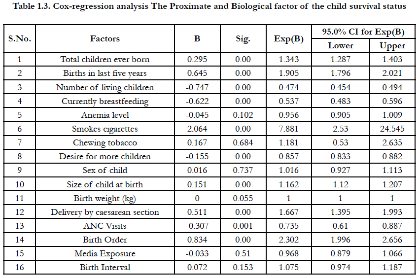
Table 1.3. Cox-regression analysis The Proximate and Biological factor of the child survival status.
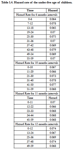
Table 1.4. Hazard rate of the under-five age of children.
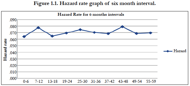
Figure 1.1. Hazard rate graph of six month interval.
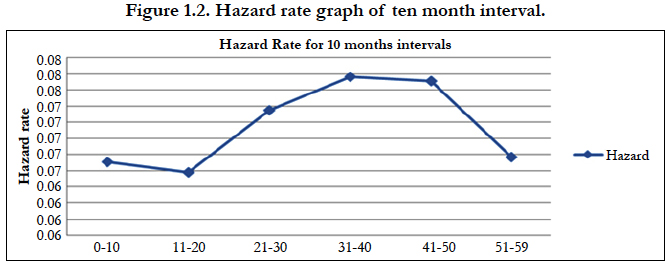
Figure 1.2. Hazard rate graph of ten month interval.
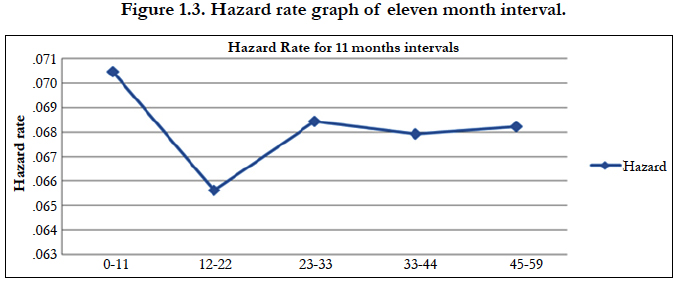
Figure 1.3. Hazard rate graph of eleven month interval.
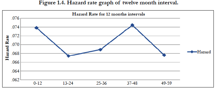
Figure 1.4. Hazard rate graph of twelve month interval.
The model breaks the data into pieces, where may fit constant hazards within these pieces .The hazard function value comes between defined pieces or interval time in months of all patients. For specifying the model with a smooth hazard function, the follow-up period was divided in 7 consecutive intervals of 59 months length. Covariates effect is calculated and represented in the graph. In the model chooses important variables which were found through Cox-regression analysis and the parameters for checking the effect of survival status.
The first piecewise hazard model includes educational level religion and women's age in years for the analysis of child survival status. This model breaks the data into pieces, where may fit constant hazards within these pieces. The table 1.5 shows the piecewise constant hazards model and find out educational level and women's age is found to be significant factor in piecewise hazard model. Figure 1.5 describe the detail of first model including covariates with a piecewise constant hazard function, piecewise constant cumulative hazard function, piecewise constant density function and piecewise constant survivor 7 consecutive intervals till 59 months. In this figure peak of the hazards continuously increasing respect to increasing time.
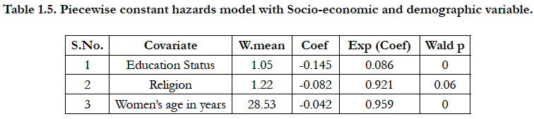
Table 1.5. Piecewise constant hazards model with Socio-economic and demographic variable.
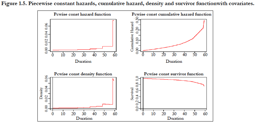
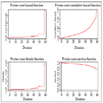
Figure 1.5. Piecewise constant hazards, cumulative hazard, density and survivor functionwith covariates.
The second model includes proximate and biological factor for under-five child mortality.
Table 1.6 shows the significant proximate and biological factors which are found through Cox-regression analysis. All variables are found to be statistically significant in the Cox-regression analysis and also found statistically significant in piecewise constant hazards model of the child mortality status. Figure 1.6 shows the piecewise constant hazard function, piecewise constant cumulative hazard function, piecewise constant density function and piecewise constant survivor 7 consecutive intervals till 59 months including proximate and biological factors.
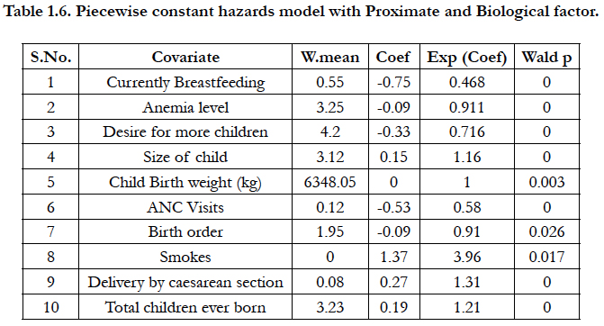
Table 1.6. Piecewise constant hazards model with Proximate and Biological factor.
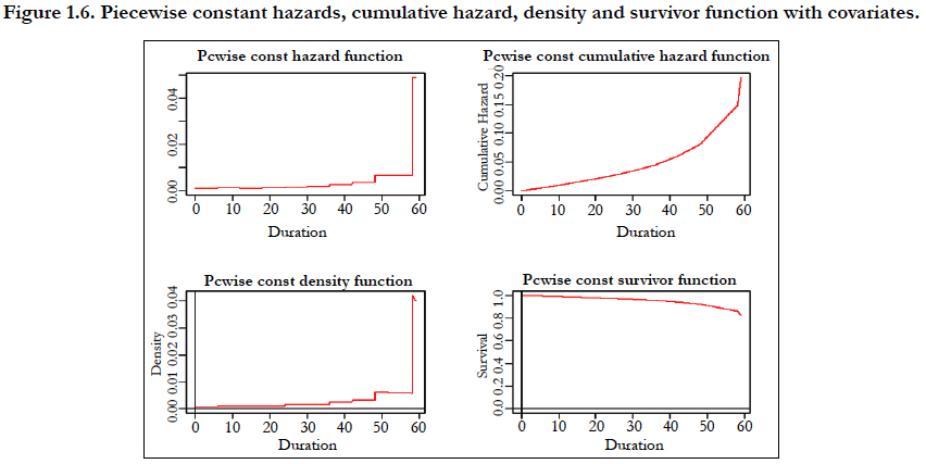
Figure 1.6. Piecewise constant hazards, cumulative hazard, density and survivor function with covariates.
Finally selected all significant factors and combined together to check effect of the factors in under-five child mortality. Table 1.7 shows that the factors women's age in years, total children ever born, birth in last five years, number of living children, present breastfeeding, smoking, desire for more children, size of child, delivery by caesarean section, ANC visits and birth orders have played significant role in under-five child mortality in the pricewise constant hazard model. Figure 1.7 describes the piecewise constant hazard function, piecewise constant cumulative hazard function, piecewise constant density function and piecewise constant survivor 7 consecutive intervals till 59 months including all combine factors.
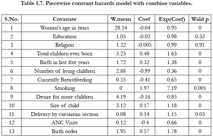
Table 1.7. Piecewise constant hazards model with combine variables.
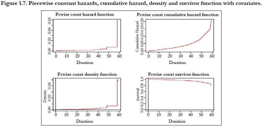
Figure 1.7. Piecewise constant hazards, cumulative hazard, density and survivor function with covariates.
Discussion and Conclusion
In survival analysis, when interest is to estimate the hazard rate, an essential and popular model is the piecewise constant hazard model. This model is easy to calculate as the hazard rate is supposed to be constant on some pre-defined time intervals and plotting the hazard rate gives a quick idea of the progress of the event of interest through time. Different time periods for appraisal of mortality, extending from 28 days to a half year and including 35 days, 60 days, and 90 days, have been utilized in earlier clinical trials [12], while this model can be utilized in a nonparametric setting, usually utilized in mix with covariates impacts [13]. This is the situation for example for the popular Poisson regression model [14] and accept a relative impact on the covariates and a piecewise constant hazard model for the baseline hazard [15]. Proposed an imaginative strategy to appraise the hazard rate in a piecewise constant model. This technique gives a programmed strategy to locate the number and location of cut points and to estimate the hazard on each cut interval. Utilized the piecewise hazard model to fit for under-five child mortality data of Uttar Pradesh which was taken from NFHS-IV. This model is exceptionally helpful to find the patient hazard in various time points and this technique actualizes and assumes a critical job in the survival models particularly different occasions cut points.
First time piece-wise constant hazard model has used for finding the crucial month period and influenced factors in under-five child mortality. In this study utilize add up to three models to evaluate our outcome through piecewise hazard model and portray the critical factor for our study. In study found that proximate and biological factors are more critical for the child mortality and half year or six months are extremely urgent for children till completing the five years of age, these outcomes can advise the determination of time points for evaluating survival status of under-five children mortality. This model can useful in health care policy decisions and with an upgraded comprehension of the adjustments in population death rates can recognize gaps, seek solutions, improve performance, and ultimately, better the public’s health.
References
- Kaplan EL, Meier P. Nonparametric estimation from incomplete observations. Journal of the American statistical association. 1958 Jun 1;53(282):457-81.
- David CR. Regression models and life tables (with discussion). Journal of the Royal Statistical Society. 1972;34(2):187-220.
- Gijbels I, GürlerU. Estimation of a change point in a hazard function based on censored data. Lifetime Data Anal. 2003 Dec; 9(4): 395-411. PMID: 15000412.
- . Kim H-J, Fay MP, Feuer EJ, Midthun DJ. Permutation test for joinpoint regression with application to cancer rates.Statist. Med. 2000 Feb 15;19(3):335-51. PMID: 10649300.
- Melody S. Goodman, Yi Li, Ram C Tiwari. Detecting multiple change points in piecewise constant hazard functions. J Appl Stat. 2011 Jan 1; 38(11):2523-2532. PMID: 22707842.
- Li Y, Gail MH, Preston DL, Graubard BI, Lubin JH. Piecewise exponential survival times and analysis of case‐cohort data. Statistics in medicine. 2012 Jun 15; 31(13):1361-8.
- Gijbels I, Gürler Ü. Estimation of a change point in a hazard function based on censored data. Life time Data Anal. 2003 Dec; 9(4): 395-411. PMID: 15000412.
- Laaksonen MA, Knekt P, Härkänen T, Virtala E, Oja H. Estimation of the population attributable fraction for mortality in a cohort study using a piecewise constant hazards model. American journal of epidemiology. 2010 Mar 2; 171(7):837-47. PMID: 20197386.
- Bouaziz O, Nuel G. Regularization for the Estimation of Piecewise Constant Hazard Rates in Survival Analysis. Applied Mathematics. 2017; 8: 377-394.
- Saroj RK, Murthy KN, Kumar M. Survival analysis for under-five child mortality in Uttar Pradesh. Int J Res Anal Rev. 2018;59:782-9.
- Mosley WH, Chen LC. An analytical framework for the study of child survival in developing countries. Population and development review. 1984 Jan 1;10(0):25-45.
- Ronco C, Bellomo R, Homel P, Brendolan A, Dan M, Piccinni P, et al. Effects of different doses in continuous veno-venous haemofiltration on outcomes of acute renal failure: A prospective randomised trial. Lancet 2000 Jul 1; 356(9223): 26-30. PMID: 10892761.
- Gastaldello K, Melot C, Kahn RJ, Vanherweghem JL, Vincent JL, Tielemans C. Comparison of cellulose diacetate and polysulfone membranes in the outcome of acute renal failure. A prospective randomized study. Nephrology Dialysis Transplantation. 2000 Feb 1; 15(2): 224-30.
- Clayton D, Hills M. Statistical models in epidemiology. OUP Oxford; 2013 Jan 17.
- Aalen O, Borgan O, Gjessing H. Survival and event history analysis. Statistics for Biology and Health. Springer. 2008; 53: 1475-84.