Simulating the Dynamic Behavior of Active Atructures
Fritsche D*
Faculty of Mechatronics and Electrical Engineering, Esslingen University of Applied Science, 73037 Göppingen, Germany.
*Corresponding Author
Fritsche D,
Faculty of Mechatronics and Electrical Engineering,
Esslingen University of Applied Science, 73037 Göppingen, Germany.
E-mail: david.fritsche@hs-esslingen.de
Received: September 23, 2019; Accepted: October 25, 2019; Published: October 31, 2019
Citation: Fritsche D. Simulating the Dynamic Behavior of Active Atructures. Int J Mechatron Autom Res. 2019;2(1):8-12.
Copyright: Fritsche D© 2019. This is an open-access article distributed under the terms of the Creative Commons Attribution License, which permits unrestricted use, distribution and reproduction in any medium, provided the original author and source are credited.
Abstract
At Esslingen University of Applied Science a simulation application is being developed called Sim2d. With this software mechanical structures can be designed and solved as static or dynamic models. The software is used in typical engineering courses such as engineering mechanics, dynamics and simulation. Because these courses are part of the study program of mechatronics and electrical engineering,the application was modified to simulate mechatronic systems. Using an active beam as example (i.e. a beam that is coupled with a control loop to minimize its deflection at the load point) this paper describes the dynamic behavior of such a system. This allows gaining insights into both the underlying mechanics and control engineering and the coupling between those two. Although the mentioned example is simple, its dynamic behavior could hardly be predicted without simulation. Furthermore, this is not just an academic problem, but could be a real industrial use case. Active structures are always desirable when high precision (i.e. positioning) and lightweight construction with corresponding low stiffness are required. For example this could be the case in the manufacturing industry, when milling processes are considered.
2.Sim2d
3.Active Structures
4.Static Model of the Traditional Beam
5.Modal Analysis of the Traditional Beam
6.Dynamic Model with Damping of the Traditional Beam
7.Dynamic Model with Damping of the Active Beam
8.Conclusion
9.References
Keywords
Finite-Element-Method, Simulation, Dynamics, Active Structures.
Sim2d
Sim2d is an application for simulating mechanical systems that is being developed at Esslingen University of Applied Sciences in Germany. The current version 1.3 is available at the following URL: www.hs-esslingen.de/~dfritsch. The benefits of the software are its easy-to-use concept and the clear visualization of results. It is especially suitable for beginners in the field of mechanical analysis and simulation. The software is intended to be used as an add-on to typical engineering courses like engineering mechanics or dynamics. It can be used by both lecturers and students.
The concept behind Sim2d is to have anapplication for teaching/learning. That is also the reason for its restriction to 2d problems. Users will understand that they can transfer the simulated mechanical principles to 3d. The software was developed completely in Java without using any platform dependent code. So in principle, Sim2d should run on any device as long as a Java runtime environment is installed.
While the successful usage of common simulation software needs a lot of training, using Sim2d is rather simple. The user defines a mechanical system in the GUI that shows a modifiable raster. The system consists of trusses, springs, beams or several 2d areas. These again can be modified, copied, merged or split, so that complex structures can be modeled. The parts of the structure can be joined together by special connectors like hinges. Furthermore it is possible to define supports, prescribed displacements and forces that act on the structure. These can also be time dependent. Finally, contact areas can be specified, so that parts of the system cannot penetrate each other.
The solver is integrated into the software and can be started from the GUI. Any problem with the model or wrong definitions will be shown in the solver log. For typical problem sizes the solver is fast enough that results are available within several seconds. As soon as the model is solved successfully, the user can visualize the results. It is possible to show deformations, stresses and forces dependent on time or as animation. For users that are interested in simulation principles the matrices used by the solver can be shown.
Because modeling, solving and visualization of results are done from the same GUI, users can change the model easily to study the effects. This can be helpful to understand the principles of mechanics.
Currently each mechanical structure can be solved as static or dynamic problem. Additionally, modal analyses are also possible. The solver is based on the method of finite elements [1-3]. Several numerical methods are implemented to fulfill the defined boundary conditions. These are the Lagrange multiplier method, the penalty method and the remove rows/columns method. The penalty method requires the specification of a penalty factoras long as the default value is not used. The remove rows/columns method does only work for simple models.
Active Structures
Mechanical structures - that may consist of several connected parts - are called active structures, if they are capable of actively responding to loads. An active response means that the structure e.g. changes its geometry or that additional counterforces are acting.
For example an active beam does not simply bend under a load, but it fights against the bending. That does not mean the active beam can carry a higher load (this would only be true in the case of suppressed buckling). But an active beam could have a defined deflection at a certain position (Figure 1). This is important for applications where high precision is required. Instead of using a traditional beam with high stiffness (which would be of heavy weight), it is possible to use an active beam with low stiffness (which would be a lightweight construction).
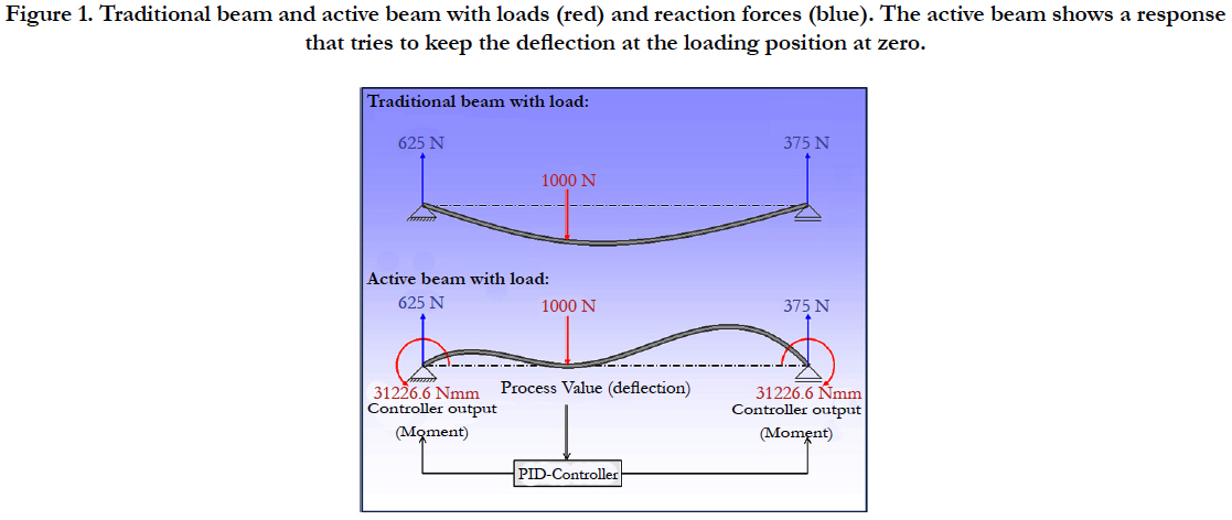
Figure 1. Traditional beam and active beam with loads (red) and reaction forces (blue). The active beam shows a response that tries to keep the deflection at the loading position at zero.
The response of an active structure is a dynamic process. The structure will deform under the load, while the measured deflection is used to calculate the controller output that modifies the structure. So every time the load changes, it takes some time until the final response of the structure is achieved. In the meantime the structure will oscillate around the final response. This is of special interest in many cases: How fast is the response with the given settings? What is the maximum deviation from the set point? In the beam example the set point is to have zero deflection at the position of the load.
To answer these questions a dynamic simulation of the active beam including the control loop can be used. In the following this simulation model is developed step by step.
Static Model of the Traditional Beam
This is a simple model to start with. We will use an Euler-Bernoulli type beam with linear kinematics. The beam has a statically determined support configuration. Material is linear elastic and the cross section is a hollow rectangle. The load is a single force at the midpoint of the beam with a bilinear time dependency (Figure 2).
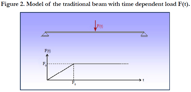
Figure 2. Model of the traditional beam with time dependent load F(t).
For the following investigation we will use the set of parameters given in Table 1. The material of the beam is assumed to be polyvinyl chloride (PVC). The material data and the damping ratio are estimated. The load is applied in 0.01 s, so this is like an impact.
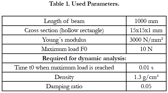

Table 1. Used Parameters.
However, in the static analysis this has no influence.
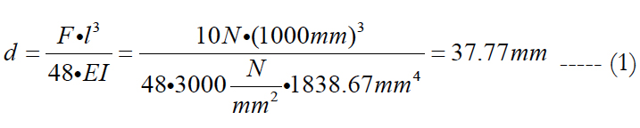
The maximum displacement will occur at the midpoint of the beam and the analytical solution is given by equation (1):
Sim2d shows the same result for the static model. In the following a plot of the vertical displacement of the midpoint of the beam over time is used. In Sim2d displacements pointing upwards are positive, hence the displacement in the plotis negative (Figure 3).
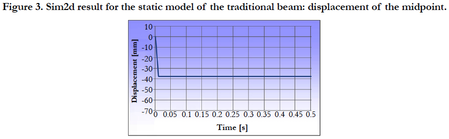
Figure 3. Sim2d result for the static model of the traditional beam: displacement of the midpoint.
Modal Analysis of the Traditional Beam
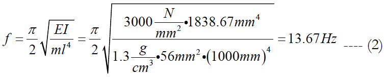
Now a modal analysis is performed. The resulting eigenmodes of the beam are used to find the input for the damping model. Here only the first two eigenmodes (corresponding to the lowest and the second lowest eigenfrequency) are of interest (Figure 4). The lowest eigenfrequency is found at 13.73 Hz, the second lowest is 60.7 Hz. The lowest eigenfrequency of a beam is given by the analytical equation (2), showing that the numerical result calculated by Sim2d is quite close.
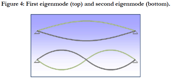
Figure 4: First eigenmode (top) and second eigenmode (bottom).
Dynamic Model with Damping of the Traditional Beam
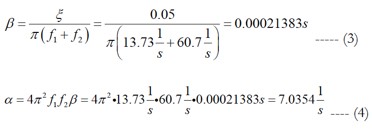
For the dynamic simulation a Rayleigh damping model is used [4]. The coefficients α and β are calculated with the damping ratio ξ and the eigenfrequencies f1 and f2 from the modal analysis in equations (3) and (4).
With these coefficients a dynamic simulation with damping can be done. The displacement of the midpoint of the beam over time is plottedin Figure 5. Now we see that the beam oscillates around the solution of the static model and that the amplitude gets smaller with time due to the damping.
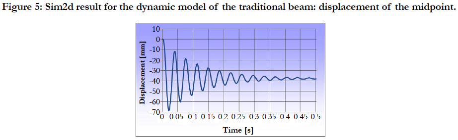
Figure 5: Sim2d result for the dynamic model of the traditional beam: displacement of the midpoint.
Dynamic Model with Damping of the Active Beam
Finally the beam is transformed into an active beam by adding the control loop. The measured process value is the displacement at the midpoint of the beam. We use a PID-controller with the settings given in Table 2. The set point of the controller is zero, which means the displacement at the midpoint should aim towards zero.
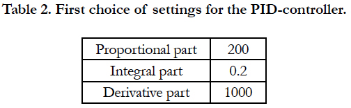
Table 2. First choice of settings for the PID-controller.
The PID-controller calculates the controller output, which is a moment applied at both ends of the beam in opposing directions. With these settings we get a displacement of the midpoint over time as shown in Figure 6. We still see oscillations in the result, which in this case are caused by the dynamic model and the control loop. The amplitude decreases and the final value is around zero, which is the set point.
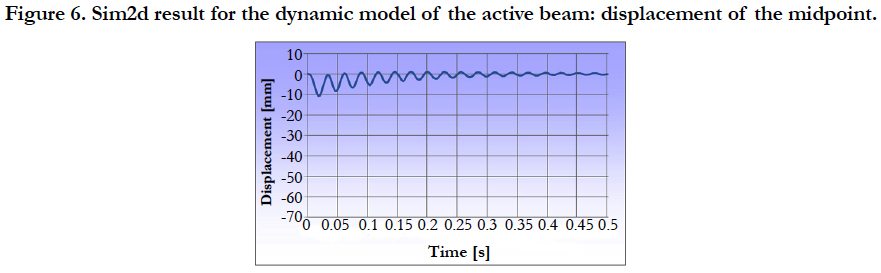
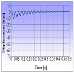
Figure 6. Sim2d result for the dynamic model of the active beam: displacement of the midpoint.
It is common practice to find the settings for the controller by trial and error with some general rules [5]. If we modify our settings corresponding to table 3, we are getting the final response even faster (Figure 7).
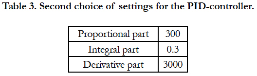
Table 3. Second choice of settings for the PID-controller.
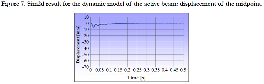
Figure 7. Sim2d result for the dynamic model of the active beam: displacement of the midpoint.
This allows trying different sets of parameters until the dynamic response of the active structure is satisfying for the current use case. If no such set of parameters can be found, we have to rethink some of the other conditions. For example the time of the load application is crucial and could possibly be less impact-like.
In Figure 8 we can see the final result for the active beam after the oscillation is decayed. The displacement in the midpoint is nearly perfectly zero and the moment at the endpoints is 1666.6667 Nmm. Compared to analytical calculations the simulation resultsfrom dynamic models tend to be less perfect due to numerical noise.
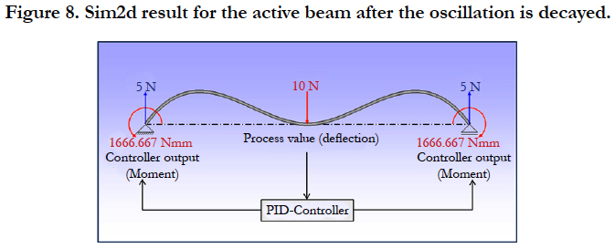
Figure 8. Sim2d result for the active beam after the oscillation is decayed.
Conclusion
Sim2d with its built-in modifications provides easy access to the simulation of active structures. Parameter studies can be carried out to gain a better understanding of the behavior of such systems. The design of control loops is not an implemented feature in the current version 1.3 of Sim2d. For the investigation under discussion in this paper the control loop was realized by modifications directly in the source code. A more convenient way of adding control loops to mechanical models is planned for future releases.
The purpose of this study is not to find the optimum controller parameters. There are several methods known in control engineering that could be used for that [5]. Furthermore, it is important to note that the proposed model does not contain any delay by the control loop (i.e. from sensors, actuators, processing or communication). It is assumed that any delay of that kind will be small and will have no significant influence on the results. To validate the results of this investigation in the future a real active beam with the proposed settings is yet to be built.
Finally, it remains to be determined, where the usage of active structures could have a benefit. With a sufficiently fast dynamic response an active structure could be used, which would be light and slim. This could be of interest for the manufacturing industry, when milling processes are considered. Instead of heavy constructions with high stiffness, milling machines could be light and of high precision.
References
- Steinbuch R. Finite Elemente - Ein Einstieg. Springer - Verlag Berlin Heidelberg; 2013 Mar 7.ISBN 978-3540631286.
- Thieme D . Introduction to the Finite Element Method for Civil Engineers. Publishing House for Construction,Berlin;1990.
- Belytschko T, Liu WK, Moran B, Elkhodary K. Nonlinear finite elements for continua and structures. John wiley & sons; 2013 Nov 25. ISBN 978- 0471987741.
- CADFEM Wiki .Rayleigh damping Category [cited 11 August 2016]. Available from: http://www.cae-wiki.info/wikiplus/index.php/Rayleigh-D%C3%A4mpfung
- Wikipedia, Rule of thumb procedure (automation technology). [cited 16 August 2019]. Available from: https://de.wikipedia.org/wiki/Faustformelverfahren_(Automatisierungstechnik).