Study on Bifurcation of H-H Parameters And Its Variants Contribution To Neurology
Taslima Ahmed*, Jiten Ch. Dutta
Department of ECE, Tezpur University (a Central University), Napaam Post, Tezpur, Assam, India
*Corresponding Author
Taslima Ahmed,
Department of ECE,
Tezpur University (a Central University),
Napaam Post, Tezpur, Assam,India.
E-mail: ahmed.taslima@gmail.com
Article Type: Research Article
Received: July 30, 2014; Accepted: July 22, 2014; Published: July 24, 2014
Citation: Taslima Ahmed, Jiten Ch. Dutta(2014) Study on Bifurcation of H-H Parameters And Its Variants Contribution To Neurology. Int J Comput Neural Eng, 1(2) 6-10. doi: dx.doi.org/10.19070/2572-7389-140002
Copyright: Taslima Ahmed© 2014. This is an open-access article distributed under the terms of the Creative Commons Attribution License, which permits unrestricted use, distribution and reproduction in any medium, provided the original author and source are credited.
Abstract
The important application of bifurcation analysis of a system is estimated by the variables of H-H model. Graphical User Interface (GUI) is essential for proper visualization of results and therefore, here, we are discussing some GUI based bifurcation panels. Based on these panels, we can investigate different abnormal disorders for neurological applications.
2.Introduction
3.Analysis of bifurcation in some models
3.1 GUI Morris- Lecar (ML) model by B.Raesi
3.2 Jiang Wang bifurcation for gl value
3.2 Jiang Wang for non-linear model
4.Conclusion
5. References
Keywords
H-H model; Bifurcation; Neurology.
Introduction
Neuron is the fundamental unit for transmitting signals in nervous system [1-3]. The biological membrane is also played an important role in many of life’s processes [4].Many of these processes are electrical and the different electrical behavior of nerve cells can be measured experimentally. The flow of ions across the membrane is responsible for the production of membrane potential. The mathematical formulation of the function of neuron was given firstly by H-H model [5-8]. The variation of parameters of H-H equations leads to bifurcation which refers to quantitative changes in the solution structure of dynamical systems.
Neuroscience computes different problems based on neural model from the analysis of bifurcation in H-H variables. This analysis progress in modern quantitative biology and biophysics [9].
It is the main significant issue to control bifurcation because many neuronal disorders are due to bifurcation of neuronal systems. In the field of neurology, these disorders present Alzheimer’s disease epilepsy and arrhythmia [10,11]. Bifurcation control has been employed to estimate seizing behavior in the model system of human cortical electrical activity [12].
In this paper, firstly we describe the GUI Morris- Lecar baesd [13] model for global phase portraits. Secondly, we show GUI panel based on the analysis by Jiang Wang [14] that finds the bifurcation would occur when the leakage conductance gl is lower than 0.299406mS/cm2. Thirdly, we again show the analysis by Jiang Wang [15] for the investigation of the synchronization of Fitz- Hugh-Nagumo neural system under external electrical stimulation via the nonlinear control by using GUI. Lastly, we discuss the application of H-H variants for contribution in neuroscience based on these example panels.
Analysis of bifurcation in some models
From this table-1, we discuss different bifurcation analysis as follows:
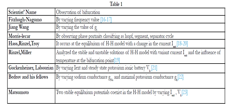

Table 1:
17],[18-20],19,21,22,23
In this ML model, to solve the equation 1, we first need to create functions m∞(v) and n∞(v). With the help of these functions, we take the different values of different parameters for plotting the various sub panels. Again, with the help of MATLAB library function “ode 23”, we solve all the differential equations2, 3, 4, 5.The solutions are plotted by taking the different values from the table-2. We plot the result of main function capacitive function Cv w. r. t time, n w. r. t time, m w. r. t time respectively. Then the different phase portraits are obtained by plotting the graph by taking three variable Cv, n, m, w. r. t each other as shown in plot (a), plot (b). The equations are shown as:
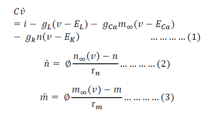
Where
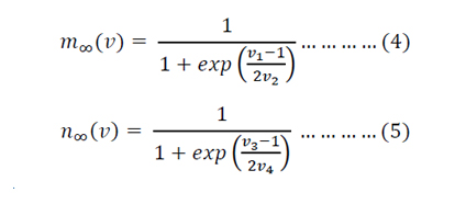
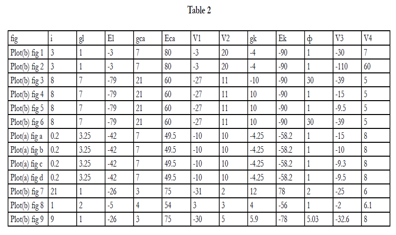
Table 2:
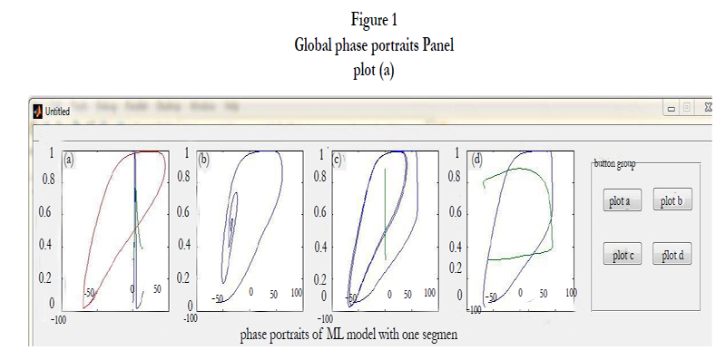
Figure 1. Global phase portraits Panel: plot (a)
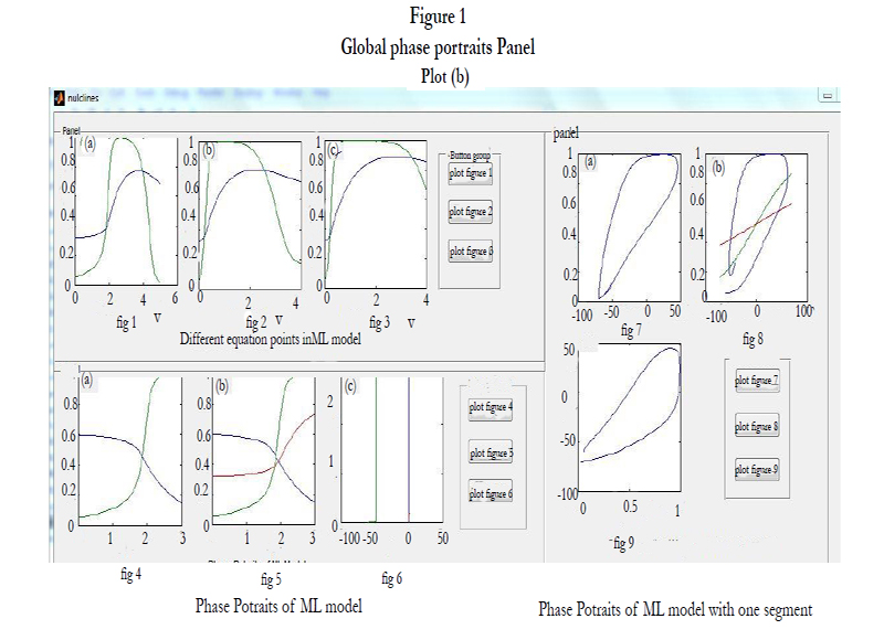
Figure 1. Global phase portraits Panel plot (b)
The HH model can be described using following four equations:
dm/dt= fm(V,m)=αm(V) (1-m)-βm (V)m
dh/dt= fh(V,h)= αh(V) (1-h)-βh(V)h
dn/dt= fn(V,n)= αn(V) (1-n)-βn(V)n
where, αm= 0.08 (V+56)/(1-exp(-(V+56)/6.8)
βm = 0.8exp(-(V+56)/18)
αh= 0.006exp(-(V+41)/14.7)
βh= 1.3 /(1+exp(-(V+41)/7.6)
αn= 0.0088 (V+40)/(1-exp(-(V+40)/7)
βn = 0.037exp(-(V+40)/40)
Where, V=membrane voltage, Iext =injected current, n=activation variable of potassium channel, m=activation variable of sodium channel, h=inactivation variable of sodium channel, Cm=1.9μF/cm2, gna=50 mS/ cm2, gk=22 mS/ cm2, gl=0.4 mS/ cm2, vna=50V, vk=-70V,vl=-81V.
By putting all the parameter’s value, we can find that there is only one bifurcation parameter which is gl..So to analyze the effect the leakage current parameter gl .We did the partial differentiation of above four equations and obtains a Jacobian matrix as shown:
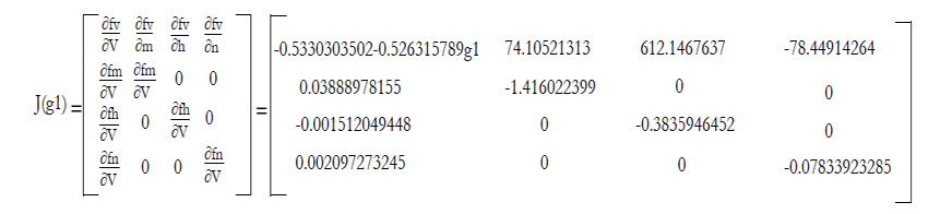
So the coefficients of Jacobian matrix are the solution find the partial differentiation of those equations and putting all values of parameters.
In the nonlinear cable model, the model equation is a coupled differential equation.
We use “ode15” function in MATLAB to solve these equations. After solving the equations the solution is plotted with respect to time having different frequencies as shown in figure-2.

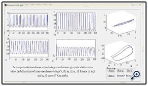
Figure 2. Jiang Wang bifurcation for gl value
The non linear model equations are given as follows with transmembrane voltage V along the nerve fibre as:
dX/dt= X(X-1)(1-rY)-Y+I(t)
dY/dt=bX
where
X,Y are membrane voltages, W=recovery variable
vp=peak of action potential
X=V/ vp, Y=W/ vp, r= vp/vT, where, vT=threshold membrane voltage
I(t)=A/ᴡ coswt, A=strength of applied field
W=angular frequency of applied field,
w=2ᴨf, f=frequency
Different observations at different frequency values are concluded with table-3 form the plot figure-3
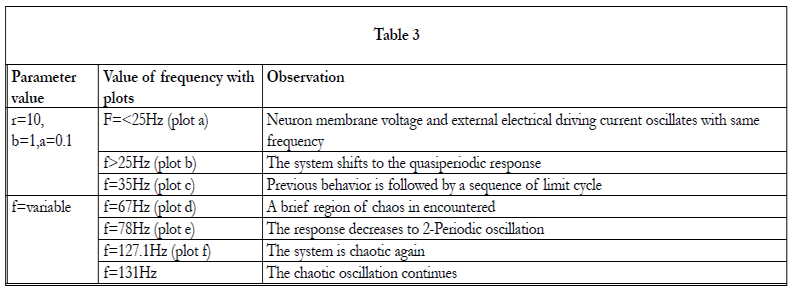
Table 3:
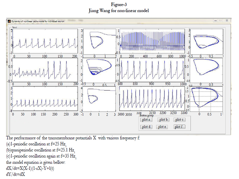
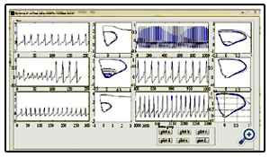
Figure 3. Jiang Wang for non-linear model
The performance of the transmembrane potantials X with various frequency f:
(a)1-periodic oscillation at f=25 Hz1MB
(b)quasiperiodic oscillation at f=25.1 Hz1
(c)1-periodic oscillation again at f=35 Hz1
the model equation is given bellow:
dX/dt=X(X-1)(1-rX)-Y+l(t)
dY/dt=dX
Understanding complex neurobiological systems is one of the most difficult challenges in modern science [24]. From these above results and discussion, we can conclude that H-H equation is the foundation of neuroscience as these parameters values are used for computational brain modeling. It removes ambiguity from theories and makes them logically consistent. Use of computer technology enables theories involving with a large number of elements to be investigated. Computational modeling can help to do the right experiment to solve numerically a set of biologically grounded equations describing the voltage-dependent changes. Computer modeling is an essential component of the neuroscientist’s repertoire. Any variation of the H-H parameters can cause bifurcation and this analysis can solve different abnormal disorders by investigating the graphs as shown above. Without H-H model, there is no existence of research in neuroscience as today. So, from these different panels based on H-H equations can solve the problem of investigation of different diseases by researchers also.
References
- Adam Kepecs, Xiao-Jing Wang, and John Lisman (2000) “Bursting neurons signal input slope,” Neurocomputing, vol. 22, pp. 9053-9062.
- Martin ST-Hilaire, Andr E Longtin (2004) “Comparison of coding capabilities of Type I and Type II neurons,” J Comput Neurosci, vol. 16, pp. 299-313.
- E. M. Izhikevich (2005) Dynamical systems in neuroscience: the geometry of excitability and bursting, The MIT Press.
- Hoppensteadt FC (1986)An introduction to the mathematics of neurons. New York: Cambridge University Press.
- A. Hodgkin, A. Huxley (1952) Currents carried by sodium and potassium ions through the membrane of the giant axon of Loligo, J. Physiol. (London) 116, 449-472.
- A. Hodgkin ,A. Huxley (1952) The components of membrane conductance in the giant axon of Loligo, J. Phsyiol. (London) 116, 473-496.
- A. Hodgkin ,A. Huxley (1952) The dual effect of membrane potential on sodium conductance in the giant axon of Loligo, J. Physiol. (London) 116, 497-506.
- A. Hodgkin and A. Huxley (1952) A quantitative description of membrane current and its application to conduction and excitation in nerve, J. Physiol. (London) 117, 500-544.
- W. Howell, N.H. Goddard and E. De Schutter (2002) ``Noncurated distributed databases for experimental data and models in neuroscience'', Network: Computation in Neural Systems 13:415—428.
- Durand, D.M., Bikson, M (2001): Suppression and control of epileptiform activity by electrical stimulation: A review. Proc. IEEE 89, 1065–1082 .
- Fröhlich, F, Jezernik, S(2004): Feedback control of Hodgkin–Huxley nerve cell dynamics. Control Eng. Pract. 10, 008–019.
- J. Rinzel (1978) One Repetitive Activity in Nerve. Fed Proc., vol. 37, 2793- 2802.
- B. Raesi (2012) classification of Global Phase Portraits of Morris-Lecar Model for Spiking Neuron,Advanced Studies in Biology, Vol. 4, no. 4, 175 – 194.
- Jiang Wang, Liangquan Chen, Xianyang Fei (2007) “Analysis and control of the bifurcation of Hodgkin–Huxley model,” Chaos, Solitons & Fractals, vol. 31, no. 1, 247–256.
- Wang, Jiang; Zhang, Ting; Deng, Bin (2007) Synchronization of FitzHugh– Nagumo neurons in external electrical stimulation via nonlinear control. Chaos, Solitons and Fractals vol. 31 issue 1 January. 30-38.
- FitzHugh R (1961) “Impulses and physiological states in theoretical models of nerve membrane,” Biophysical J. vol. 1, pp. 445-466.
- Nagumo, J., Arimoto, S., Yoshizawa, S (1962)“An active pulse transmission line simulating nerve axon,” Proc IRE. vol. 50, pp. 2061–2070.
- [Hassard B (1978) Bifurcation of periodic solutions of the Hodgkin–Huxley model for the squid giant axon. J Theor Biol;71:401–20.
- Rinzel J, Miller RN (1980) Numerical calculation of stable and unstable solutions to the Hodgkin–Huxley equations. Math Biosci;49:27–59.
- W.C. Troy (1978) The Bifurcation in the Hodgkin-Huxley Equations. ApplMath. Q., vol. 36, pp 73-83.
- J. Guckenheimer ,I.S. Labouriau (1993) Bifurcation of the Hodgkin and Huxley Equations: a New Twist, Bull. Math. Biol., vol. 55, pp 937-952.
- Y.A. Bedrov, G.N. Akoev ,O.E. Dick (1992) Partition of the Hodgkin- Huxley Type Model Parameter Space in to the Region of Qualitatively different solutions. Biol Cybern;66:413–8.
- K. Aihara ,G. Matsumoto (1983) Two Stable Steady States in the Hodgkin- Huxley Axons, Biophys. J., vol. 41, pp 87-89.
- David Sterratt, Bruce Graham, Andrew Gillies David Willshaw (2011) Principles of Computational Modeling in Neuroscience,Cambridge University Press, Cambridge, UK; ISBN: 978-0-521-87795-4; Hardback; 390 .