Modeling The Mysterious Tsunami Swirls In The Northeast Coast Of Japan During The March 2011 Tohoku Earthquake
Paul C. Rivera*
Hymetocean Peers Co., Antipolo City, Philippines.
*Corresponding Author
Paul C. Rivera,
Hymetocean Peers Co., Antipolo City, Philippines.
Tel: +632-86465730
E-mail: pcrivera@gmail.com
Received: January 09, 2020; Accepted: March 19, 2020; Published: March 28, 2020
Citation: Paul C. Rivera. Modeling The Mysterious Tsunami Swirls In The Northeast Coast Of Japan During The March 2011 Tohoku Earthquake. Int J Marine Sci Ocean Technol. 2020;7(1):117-123. doi: dx.doi.org/10.19070/2577-4395-2000016
Copyright: Paul C. Rivera© 2020. This is an open-access article distributed under the terms of the Creative Commons Attribution License, which permits unrestricted use, distribution and reproduction in any medium, provided the original author and source are credited.
Abstract
The formation of tsunami swirls near the coast is an obvious oceanographic phenomenon during the occurrence of giant submarine earthquakes and mega-tsunamis. Several tsunami vortices were generated during the Asian tsunami of 2004 and the great Japan tsunami of March 2011 which lasted for several hours.
New models of tsunami generation and propagation are hereby proposed and were used to investigate the tsunami inception, propagation and associated formation of swirls in the eastern coast of Japan. The proposed generation model assumes that the tsunami was driven by current oscillations at the seabed induced by the submarine earthquake. The major aim of this study is to develop a tsunami model to simulate the occurrence of tsunami swirls. Specifically, this study attempts to simulate and understand the formation of the mysterious tsunami swirls in the northeast coast of Japan. In addition, this study determines the vulnerability of the Philippines to destructive tsunami waves that originate near Japan. A coarseresolution model was therefore developed in a relatively large area encompassing Japan Sea and the eastern Philippine Sea. On the other hand, a fine-resolution model was implemented in a small area off Sendai coast near the epicenter. The model result was compared with the tsunami record obtained from the National Data Buoy Center with relatively good agreement as far as the height and period of the tsunami are concerned. Furthermore, the fine-resolution model was able to simulate the occurrence of tsunami vortices off Sendai coast with various sizes that lasted for several hours.
2.Introduction
3.Methods
3.1 Tsunami Generation Model
3.2 Dispersive Long-Wave Tsunami Model
4.Results and Discussion
4.1 Comparison of Observed and Computed Tsunami Height
4.2 Simulated Tsunami Swirls
5.Conclusions
6.References
Keywords
Tsunami Swirls; Tsunami Generation Mechanism, Dispersive Tsunami Model.
Introduction
Tsunami swirls had been observed to occur during the occurrence and propagation of tsunami waves. Actual observations during the March 2011 Japan Tsunami and the Indian Ocean Tsunami of December 2004 showed the formation of swirls which lasted for some hours. The tsunami vortices (Figure 1) during the East Japan earthquake and tsunami of March 2011 were photographed off Iwaki coast, Fukushima Prefecture. The twin swirls lasted for several hours after the quake (www.dailymail.co.uk/sciencetech/). They also generated a loud roar.
Tsunami modeling studies conducted by previous authors dealt with the simulation of tsunami heights and inundation of coastal areas (Song 2007). The aim of this study is to develop a tsunami model to simulate the occurrence of tsunami swirls. Specifically, this study is a novel computational attempt to understand the formation of mysterious swirls in March 2011 in the northeast coast of Japan. In addition, this study determines the vulnerability of the Philippine Archipelago to destructive tsunami waves that originated in Japan.
The present study makes use of the coarse-resolution bathymetric data from NOAA-NGDC ETOPO-1 which was aggregated into a 6-km grid resolution (Figure 2). To determine the occurrence of tsunami swirls, a fine-resolution bathymetric map off the eastern coast of Sendai and Iwaki was also digitized (Figure 3).
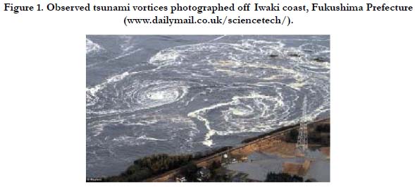
Figure 1. Observed tsunami vortices photographed off Iwaki coast, Fukushima Prefecture (www.dailymail.co.uk/sciencetech/).
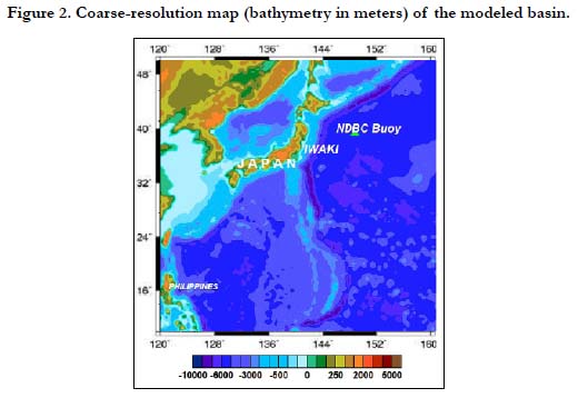
Figure 2. Coarse-resolution map (bathymetry in meters) of the modeled basin.
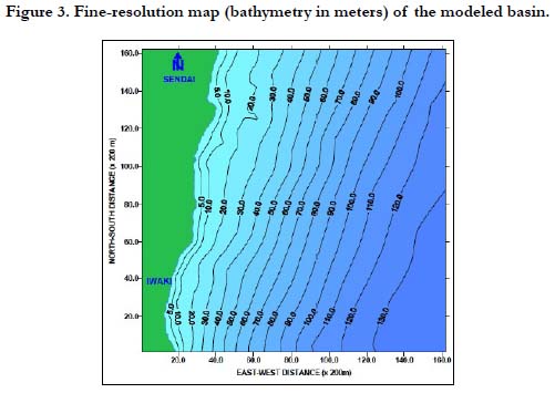
Figure 3. Fine-resolution map (bathymetry in meters) of the modeled basin.
The generation mechanism of tsunamis is still not fully understood. Tsunami occurrence had been documented during submarine earthquakes and volcanic island eruptions. Even when an earthquake epicenter is inland or at sea, some tsunamis had also been observed. Furthermore, tsunami occurrence had been documented even when the faulting mechanism is strike-slip or dip-slip. In addition, the formation of mysterious whirlpools or swirls has been documented in many areas like the coast of Thailand and Indonesia during the great Asian Tsunami of December 2004. It is therefore imperative to find a tsunami generation mechanism that can explain the formation of destructive tsunamis and associated swirls as a result of the strong seabed motion during major earthquakes.
There are two hypotheses that can be put forward in the generation of tsunamis. First, sufficient time is a necessary condition for a powerful tsunami to develop. Here, the duration of the submarine earthquake is important. When a water mass is displaced during a tsunami, it normally oscillates at the Brunt-Vaisalla (buoyancy) frequency. During a submarine earthquake or volcanic explosion, the frequency of oscillation of the horizontal currents produced in oceanic waters can be an order of magnitude higher than the Brunt-Vaisalla frequency as the natural period is determined by the water depth and gravity. This period, expressed by the square root of the local water depth divided by the gravitational acceleration, must be exceeded by the rupture duration in order for a single discernible tsunami wave to occur. A short rupture duration that is associated with fast rupture velocity may not produce a discernible tsunami in shallow or deep waters. This time requirement, coupled with the depth requirement (2nd hypothesis), could be the reason why no tsunami had been observed in a number of strong earthquakes in the past.
A second hypothesis which needs careful consideration is that, the frequency of ground motion during a seismic disturbance should match the frequency of oscillation of the water currents for a destructive tsunami to occur. The frequency of current oscillation ω is strongly dependent on the water depth, ω = 2π /Tc , where Tc is the period of current oscillation given by √h / g / 2 in which h is the water depth and g is gravitational acceleration (Rivera 2006).
The tsunami generation mechanism applied here takes these factors into consideration and can be explained in terms of a simple balance of forces. During a submarine earthquake, a strong pressure and collision force is exerted in the ocean column by the seabed (Rivera 2006). This seabed motion, whose pressure acts in all directions) should accelerate currents opposite to the direction of the applied pressure gradient force (i.e. ρ-1 ∇ Pe = −ax), where ρ is water density, Pe is seabed pressure and ax is horizontal current acceleration). It was previously postulated in Rivera (2006) that a tsunami may occur if the prevailing downward force or pressure of the ocean column is exceeded by the total force exerted by the seabed during the quake. The horizontal collision force and the associated cross-fault currents generate a tsunami during a submarine earthquake. The seabed slope plays a very important role as the magnitude and direction of the induced currents are highly dependent on it. In the case of the Japan tsunami of March 2011, strong currents should have initially flowed eastward, then oscillated westward (to and fro) above the ruptured fault. Song et al. (2006) and Song (2007) also showed using observations on the Indian Ocean mega-tsunami of 2004 that seismic-induced horizontal seabed motion did generate strong currents and tsunami waves which propagated outwards from the source region.
The impulsive motion of the horizontal currents and their succeeding convergence and divergence should produce a series of waves that radiates away from the source region. The oceanic currents produced during the submarine earthquake oscillate in time t according to:
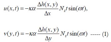
where u(x,t) and v(x,t) are the seismic-induced cross-fault current components (m/s), к is a non-dimensional tuning parameter (equal to the von Karman constant), Nz is the Brunt-Vaisalla or buoyancy frequency of the ocean column, and ω is the local current frequency given by ω = 2π/Tc, in which Tc is the period of current oscillation (i.e. duration of submarine earthquake). The bathymetric slope of the disturbed seabed is the bathymetric gradient given by (Δh/Δx).
The α-parameter is the lateral collision speed between the seabed and the ocean column during the quake. It is a very important factor that determines the magnitude of the currents and tsunami induced by the earthquake which is given by (Rivera 2006):
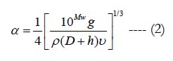
where Mw is the moment magnitude of the earthquake, D is the focal depth of the earthquake, and ν is the kinematic viscosity of seawater. The moment magnitude of the earthquake is a crucial parameter here as higher Mw values mean greater tsunami waves. The model can generate a tsunami even when the quake originates inland as some observations show. In case the epicenter is located inland, the actual focal depth D increases as 2 2 v h D = D + D where Dv is the actual focal depth directly beneath the epicenter and Dh is the horizontal distance from the epicenter. This case implies relatively lower current magnitudes for inland quakes compared with submarine quakes and lower tsunami wave heights as well. The present model therefore supports the observation that tsunamis can be generated by both submarine and inland shallowfocus earthquakes. The Erzindzhan earthquake and tsunami of December 26, 1939 in the Black Sea is an example of a tsunami that was generated by an earthquake whose epicenter was located inland (Dotsenko, 2011). The tsunami generation mechanism that is used in this study assumes a horizontal collision force of the seabed and could also be used to simulate the waves generated during volcanic eruptions. During the eruption of volcanic islands, ground accelerations in the volcanic slopes can produce oscillating currents. The ocean currents produced by the ground motion during eruption would oscillate at a frequency that is also dependent on the local water depth and the gravitational acceleration.
The period of current oscillation produced during and after the earthquake is half of the square root of the water depth divided by the gravitational acceleration as in Rivera (2006). Offshore of the Honshu source region during the March 2011 earthquake, this takes about 10 seconds assuming an ocean depth of about 4000 m. The difference between the new model and the conventional model is that the dynamic motion of the ocean column is simulated by virtue of the induced time-dependent current oscillation. When the seabed disturbance sets in, the seawater responds almost immediately as the rupture velocity goes at an enormous speed. The proposed tsunami generation model assumes that the ocean currents (given by Equations 1-2) oscillate in time with duration equal to the earthquake duration. Once set in motion, the currents would continue to oscillate even after the quake duration until dissipated by friction and gravity. It is postulated that the maximum duration of current oscillation is equal to the inverse of the buoyancy frequency (T ~ 2π/Nz). The buoyancy frequency is considered an important hydrodynamic factor in the new generation model. Nz is the frequency of oscillation for a water mass that is displaced vertically upwards during seabed displacement. It is dictated by the vertical stability and compressibility of the ocean column and is given by;
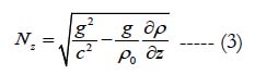
Here, c is the speed of sound in seawater (about 1485 m/s), ρo is the reference density (about 1025 kg/m3). Assuming a -3 kg/ m3 density difference from surface to bottom in a 4 km ocean depth, this gives a buoyancy frequency Nz = 0.00713 s-1. Given all earthquake parameters constant, it can be seen from Equation (1) that the stability of the water column can increase the current acceleration or velocity (and consequently, the wave heights) if the vertical stratification of the water column is stable with negative vertical density gradient giving Nz a higher magnitude. The effect of wave amplification due to ocean compressibility has been suggested by Hunt (1993).
The newly proposed tsunami generation mechanism was corroborated by Song et al. (2006) and Song (2007) which concluded that the great Asian tsunami was largely generated by a strong lateral collision force of the continental slope and the ocean column as shown by independent evidence from seismographs, satellite radar altimeters, and tide gauges in the region. Recently, Dotsenko (2011) also proposed a similar tsunami generation model with the transfer of horizontal momenta to the liquid medium via the horizontal displacements of the vertical lateral boundary of a basin. He showed that the efficiency of generation of the surface waves by the elastic displacements of the lateral boundaries of the basin is much higher than that in the case of displacements of the boundary with residual bottom deformations. Instead of using horizontal displacements, the new generation model uses the horizontal current oscillations induced by the earthquake.
Altimeter data from satellites showed that trans-oceanic megatsunamis are highly dispersive. It is therefore necessary to use a dispersive long-wave model to simulate the tsunami propagation. This study differs from previous modeling studies in that a dispersive wave model was used instead of the conventional nondispersive long-wave model. Assuming that water density does not change with time, the partial differential equation describing the time-dependent variation of the surface wave heights in the ocean area of interest is given by the mass continuity equation:
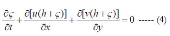
where p is the porosity, ζ is the wave height, t is time, and x and y are coordinate axes in the Cartesian system, u and v are the mean components of the wave-induced flow in the x and y axes respectively, τ s is the wind stress acting over the sea surface, ρ is the sea water density, h is the total water depth, and ho is the still water level. This time-dependent equation allows for the determination of the temporal as well as spatial variation and evolution of the wave height due to the divergence (and convergence) of the horizontal currents produced by an applied disturbance at the seabed.
The difficulty in modeling tsunami can be due to the fact that they are intermediate, quasiinfragravity waves, having the combined characteristics of long and short ocean waves. Previous authors (e.g. Koutitas and Laskaratos 1988, Pedersen et al. 2005), initiated the idea to seek a combination of a dispersive and non-dispersive wave model. The no ...n-dispersive model may be applied in the open ocean while the dispersive model could be applied in shallow coastal areas to determine the transformation of the waves as they travel from deep to shallow waters. For this reason, the nonlinear dispersive momentum equations originally proposed by Peregrine (1967) and Wu (1981) for the study of long waves in oceans and beaches were modified and applied in this study. In combination with a simple periodic current induced by a seismic disturbance, the nonlinear dispersive model used was simplified further from (Rivera 2006). The effects of ocean baroclinicity and compressibility are included by using a modified pressure term. The modified momentum conservation equations for dispersive tsunami waves used in this study take the non-linear forms:
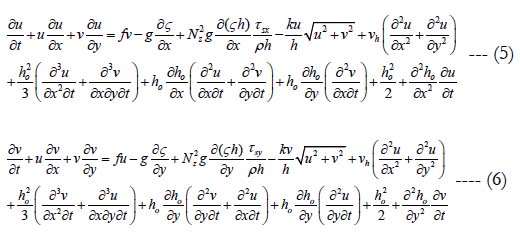
where u and v are the depth-averaged wave-induced flow components in the x and y-axes respectively, p is a porosity factor that allows for partial reflection and transmission of waves, f is the latitude-dependent Coriolis parameter, g is the gravitational acceleration, Nz is the buoyancy (or Brunt-Vaisalla) frequency, k is a frictional resistance coefficient, and υh is the horizontal eddy viscosity coefficient (assumed c constant). The total water depth h is the sum of the still water depth ho and the surface wave height ζ. As these equations represent a balance of forces in the ocean, they are useful in dealing with non-linear dispersive long and intermediate waves in both deep and shallow coastal waters. In the present study, these dispersive wave equations are applied in both deep oceanic waters and shallow coastal waters. With the addition of dynamic pressure, wind effect, and horizontal viscosity, they represent the modified two-dimensional dispersive long-wave equations in oceans and coastal waters. The eight terms to the right of the momentum equations are considered important as they describe the diffusive effect of sloping ocean bottom. They also allow lower frictional effect where high friction often obliterates the real numerical solution by unnecessary damping of the resulting current velocity field. The last two terms are deep water terms and their effects are also small but considered here to represent the propagation of the tsunami waves from deep to shallow waters. Villenueve and Savage (1993) derived a more sophisticated momentum equation taking into consideration the bed motion. The present model assumes that the sea bed is stationary and it is the ocean column that moves in a dynamic fashion during and after the seismic disturbance.
The wind stress effect was included to determine the contribution of the wind energy in the horizontal momentum dispersion and hence in the long-distance propagation of the tsunami waves. The presence of the wind can be seen in an increased horizontal currents and the interaction between the wind-driven currents and the waves may be important during a tsunami occurrence. The wind stress terms can be estimated from quadratic stress formulas found in literature (Rivera 1997). It can be seen that the pressure terms in the momentum equations consist of the sum of the hydrostatic and dynamic pressures due to a barotropic and a baroclinic ocean. This is considered important in geophysical flows with a considerable influence of vertical stability and vertical acceleration as could be the case during a tsunami. A constant wind speed of 5 m/s from the east was assumed in the present tsunami simulation. The present study did not consider the effect of a variable tide. Thus, a constant tide level of 0.5 m was added to the computed tsunami height.
The non-dimensional bottom frictional resistance k is normally taken as constant with values ranging from 0.0001-0.1. The lower limit was used in the present modeling study. The use of a very low (zero) bottom friction coefficient is made possible with the inclusion of the las term in the momentum equation. This term is subtracted from the first term, and the whole momentum equation was divided by. This was also done for the y-component of the momentum equations. The effect of the earth’s rotation (e.g. Coriolis force) on the waves was also considered in the present study by including it in the momentum equations. In higher latitudes, the Coriolis force may have a significant effect especially when horizontal currents are strong and may therefore affect the tsunami waves as they travel away from the source region.
Results and Discussion
The tsunami generation model (Equation 1-2) was initially applied in a relatively small area of about 24 km by 48 km (4 x 8) at a distance of about 50 km off the coast of Northeast Japan. It is within this area where abrupt bathymetric slope occurs. The tsunami generation model was applied in this area with a period of about 3 minutes using a constant moment magnitude of about Mw = 9.0 and focal depth of about 10 km. After the assumed quake duration, the already accelerated currents from the source area and the resulting turbulent sea column continue to oscillate and extend spatially until dissipated by gravity and friction. Nosov and Skachko (2001) initially suggested that current oscillation during ground motion is an important non-linear mechanism for tsunami generation.
In a series of numerical tests with the new dispersive long-wave model, a ‘numerical gravity’ error is observed. This kind of damping error had been documented in a series of numerical tests by Abbott et al. (1984). This was corrected in the present modeling work by applying a gravity correction term to the x and y-momentum equations respectively, in the form;
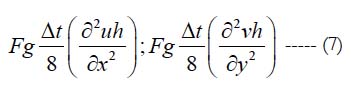
The value of F needs to be tuned and after a series of numerical simulations, the gravity error was removed. This error is seen as a progressive damping of tsunami wave height after several hours or days of numerical integration. The components of current along the x and yaxes were computed using Equations 5-6. The bathymetric slope corresponding to the u and v-components was computed for each grid along both directions x and y-axes as the absolute value of the difference between the water depths of two adjacent grid points divided by s. To maintain numerical stability and to obtain more accurate results, the time interval used in the numerical integration was 2 seconds. This was reduced to 0.5 second for the fineresolution model.
The results of the present modeling work are shown in a series of maps in Figures 4-5. It can be seen in Figure 5 that the proposed generation model would produce a complex wave pattern of positive and negative waves in the source region located almost above the ruptured fault line. The assumption of a straight fault still showed a complex wave pattern due to the complex current oscillations. The computed wave heights 10-20 minutes after the quake showed a combination of positive and negative waves radiating away from the source region (Figure 5). Negative waves shown by the blue contours are predominant east and southeast of the source region. The tsunami waves 30 minutes after the quake dispersed quite rapidly eastward. After 1 hour, a trapped wave appeared in the northeast coast of Japan while most of the tsunami waves dispersed away from the source region.
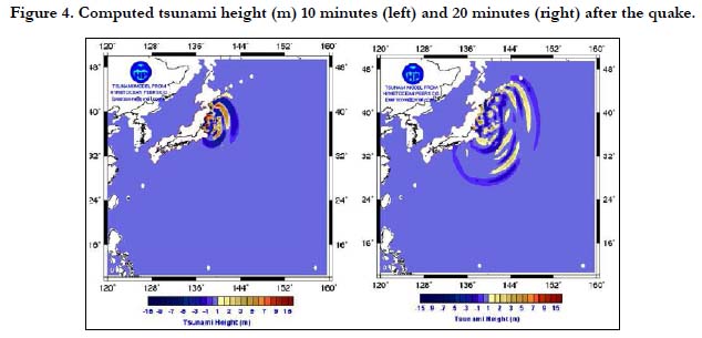
Figure 4. Computed tsunami height (m) 10 minutes (left) and 20 minutes (right) after the quake.
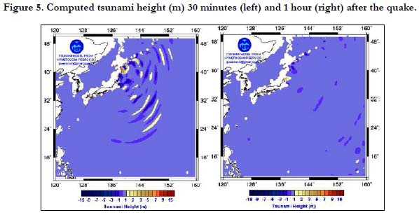
Figure 5. Computed tsunami height (m) 30 minutes (left) and 1 hour (right) after the quake.
To determine the accuracy of the newly proposed tsunami generation and propagation models, the observed tsunami height was taken from the National Data Buoy Center (http:// www.ndbc.noaa.gov/). Buoy 21418 is a 2.6 m discus buoy which recorded the data at a depth of about 5662 m (Figure 1). The depth was subtracted from the data to obtain the tsunami record. As shown in Figure 6, the computed tsunami heights in the area agree well with the observed data. The maximum tsunami height recorded at Buoy 21418 was about 2.236 m while the maximum computed tsunami height was about 2.4 m. The data in the site showed that the period between the first and second tsunami waves was about 4 minutes. This was also simulated well by the new dispersive model giving a 4-minute time period (Figure 6).
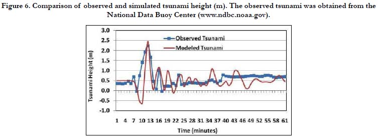
Figure 6. Comparison of observed and simulated tsunami height (m). The observed tsunami was obtained from the National Data Buoy Center (www.ndbc.noaa.gov).
Figure 7 also showed computed tsunami waves in the northern and eastern coasts of the Philippines. Less than 1 hour after the quake, the first wave with height of less than 0.4m arrived in the northern and northeast coast of the archipelago. The highest tsunami wave in the Philippines arrived after less than 2 hours in the northern coast with a height of about 0.5 m. The maximum tsunami height that reached the eastern coast of Southern Philippines was less than 0.4 m. The absence of reliable time series of tsunami heights in the Philippines during the event precludes further verification.
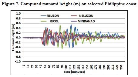
Figure 7. Computed tsunami height (m) on selected Philippine coast.
The fine resolution grid has a 200-meter spatial resolution. Using the same generation and propagation models, this was applied in the eastern coast of Iwaki, Fukushima Prefecture located south of Sendai, Japan. The simulated tsunami swirls are shown in Figures 8-11. As shown, a series of tsunami swirls was simulated by the model. Off the coast of Iwaki, several swirls were also observed which lasted for several hours. The computed maximum strength of the tsunami vortices (i.e. maximum current speed) during the first 30 minutes, 1 hour, and 2 hours after the earthquake was about 3.2 m/s, 2.3 m/s, and 1.7 m/s, respectively. The strength of the tsunami swirls gradually lost power and waned during the succeeding hours. After 4 hours, the maximum current speed of the vortices was less than 1.0 m/s. It took more than 6 hours before the swirls completely dissipated. The model also showed a reduction in the number of tsunami swirls during the succeeding hours, and a weakening of the remaining tsunami vortices.
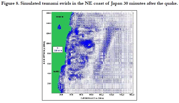
Figure 8. Simulated tsunami swirls in the NE coast of Japan 30 minutes after the quake.
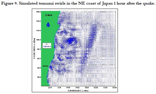
Figure 9. Simulated tsunami swirls in the NE coast of Japan 1 hour after the quake.
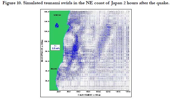
Figure 10. Simulated tsunami swirls in the NE coast of Japan 2 hours after the quake.
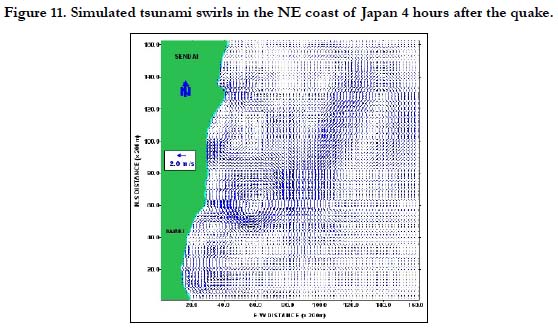
Figure 11. Simulated tsunami swirls in the NE coast of Japan 4 hours after the quake.
After 6 hours, the maximum current speed of the strongest remaining tsunami vortex computed by the model was about 0.7 m/s. It is postulated that a decreasing magnitude of horizontal currents at the surface, mid-depth and near the bottom would occur within the tsunami vortices. It was hypothesized in Rivera (2006) that the bottom currents at the source region could be stronger than at the surface. When sufficient force from the earthquake generated currents ensue, this mechanism may also cause a landslide at the seabed. However, as the tsunami propagates away from the source region, the currents become stronger at the surface than near the bottom due to frictional influence especially since the vortices mostly occur in shallow near-shore regions where friction becomes a significant component of the tsunamiinduced oceanic motion.
Conclusions
Computational dynamic models for tsunami generation and swirl propagation had been used to simulate the impact of the great Japan Tsunami of March 2011. The effects of various factors in the tsunami inception such as earthquake moment magnitude, focal depth, vertical stability of the ocean column, and bathymetric slope had been included in the new generation model. The new propagation model could account for the observed dispersive characteristics as the tsunami travel through variable ocean bathymetry and coastal geometry. With adjusted parameter values, the tsunami model could explain the independent and combined effects of various factors related to the seismic disturbance and ocean properties.
The new generation and propagation models were able to simulate the occurrence of a series of tsunami swirls in the shallow nearshore areas of Northeast Japan. In particular, the series of tsunami vortices near Iwaki coast in the Fukushima Prefecture was correctly simulated by the model. The generation model, in combination with the coupled mass continuity and newly proposed dispersive momentum equations, was successfully applied in the great Japan tsunami of March 2011.
Further calibration of the new models requires accurate information of observed swirls and currents aside from information on earthquake magnitude and focal depth, area and slope of ruptured seabed and observed wave heights. Moreover, the model can be calibrated by using observations, if any, on the strength and size of the tsunami swirls.
References
- Abbott MB, McCowan AD, Warren IR. Accuracy of short-wave numerical models. J Hydr Eng. 1984 Oct;110(10):1287-301.
- Dotsenko SF. Generation of long waves in a basin by short-term displacements of the lateral boundary. Physical Oceanography. 2011 Jul 1;21(2):75-84.
- Koutitas C, Laskaratos A. Tsunami-induced oscillations in Corinthos Bay: Measurements and 1-D vs 2-D Mathematical Models. Sci. Tsunami Hazards. 1988;6(1):51-6.
- NDBC[Internet].USA: National Oceanic and Atmospheric Administration; [cited 2020 Jan 8]. Available from: https://www.ndbc.noaa.gov/
- NGDC[Internet].USA:National Centers for Environmental Information; Available from: https://www.ngdc.noaa.gov/
- Sciencetech[Internet].UK: Available from: http://www.dailymail.co.uk/sciencetech/
- [7]. Hunt, B. A mechanism for tsunami generation. J of Hydraulic Research. 1993; 31: 111-120.
- Nosov MA, Skachko SN. Non-linear mechanism of tsunami generation by bottom oscillations. Natural Hazard and Earth Sciences. 2001(1):44-7.
- Pedersen NH, Rasch PS, Sato T. Modelling of the Asian tsunami off the coast of northern Sumatra. Danish Hydraulic Institute Technical Paper. 2005 Mar.
- Peregrine DH. Long waves on a beach. J Fluid Mech. 1967 Mar;27(4):815-27.
- Rivera PC. Modeling the Asian tsunami evolution and propagation with a new generation mechanism and a non-linear dispersive wave model. Sci Tsunami Hazards. 2006 Jan;25(1):18-33.
- Rivera PC. Hydrodynamics, sediment transport and light extinction off Cape Bolinao, Philippines. 244 p.
- Song YT. Detecting tsunami genesis and scales directly from coastal GPS stations. Geophys Res Lett. 2007 Oct;34(19).
- Song Y, Fu L, Zlotnicki V, Ji C, Hjorleifsdottir V, Shum C, Yi Y. Horizontal motions of faulting dictate the 26 December 2004 Tsunami Genesis. InAGU Fall Meeting Abstracts 2006 Dec.
- Wu TY. Long waves in ocean and coastal waters. J Eng Mech Div. 1981;107(EM3):501-22.