Dynamic Analysis of Nonlinear Stochastic Systems by Polynomial Chaos Expansion (PCE)
Lamrhari M1, D Sarsri2, Azrar L3, Rahmoune M1*, Sbai K1
1 Laboratoire d’Etudes des Matériaux Avancés et Applications, FS–EST, Université Moulay Ismail, Meknès, Morocco.
2 Laboratoire des Technologies Innovantes, ENSA, Université Abdelmalek Essaadi, Tanger, Morocco.
3 Equipe Modélisation Mathématique et Contrôle, FST, Université Abdelmalek Essaadi, Tanger, Morocco.
*Corresponding Author
Miloud Rahmoune,
Laboratoire d’Etudes des Matériaux Avancés et Applications,
FS–EST, Université Moulay Ismail,
Meknès, Morocco.
Tel: +212 661341939
E-mail: rahmoune@umi.ac.ma
Received: November 03, 2016; Accepted: December 06, 2016; Published: December 09, 2016
Citation: Lamrhari M, D Sarsri, Azrar L, Rahmoune M, Sbai K (2016) Dynamic Analysis of Nonlinear Stochastic Systems by Polynomial Chaos Expansion (PCE). Int J Aeronautics Aerospace Res, S4:001, 1-8.doi: http://dx.doi.org/10.19070/2470-4415-SI04001
Copyright: Rahmoune M© 2016. This is an open-access article distributed under the terms of the Creative Commons Attribution License, which permits unrestricted use, distribution and reproduction in any medium, provided the original author and source are credited.
Abstract
This paper deals with the analysis of the dynamic behavior of nonlinear systems subject to probabilistic uncertainties in the physical parameters. The Polynomial Chaos Expansion PCE is proposed to resolve this problem. The main objective is to estimate the probability distribution of the non linear dynamic response for a given dispersion of mass parameters. The method proposed allows notable performances in terms of efficiency and accuracy. This result comes from a comparison between the PCE performance with those offered by the Perturbation Method (PM) and the referential method Monte Carlo Simulation (MCS). This approach allows reducing the computational cost.
2.Introduction
3. Modeling of a Nonlinear Dynamical System
4. Stochastic Perturbation Method
4.1.Zero order equation
4.2.First order equation
4.3.Second order equation
5.Polynomial Chaos Expansion Method
6.Stochastic Temporal Response
7.For Perturbation Method
7.1.Zero order equation
7.2.First order equation
7.3.Second order equation
8.For Polynomial Chaos Expansion Problem
9.Numerical Example
10.Conclusion
11.References
Keywords
Non Linear Structure; Uncertain Parameters; Polynomial Chaos Expansion; Perturbation Method.
Introduction
In a robust design process, the determination of the variability of the nonlinear dynamic response of a complex structure is essential. Uncertainties come from the tolerances of manufacturing, the boundary conditions and the external excitations. These structures are largely used in the fields of aerospace, automotive, civil engineering ...The uncertainty of the physical parameters; nonlinearity and complexity of the structure require the development of a complete mathematical approach for predicting the dynamic behavior variability.
In addition, several methods have been developed in the literature to take account of uncertain parameters in the nonlinear dynamic response. The reference method is the Monte Carlo simulation [1]. This method allows a statistical evaluation based on a large number of deterministic analyses by considering different values of uncertain parameters. However, it requires the generation of big size samples then generates a prohibitory time computing. This approach is thus very costly. Also perturbation methods are widely used to calculate the first moments (mean, standard deviation) of dynamic response whose uncertain variables vary slightly. These techniques are based on the Taylor series development of the response around its mean.
This allows the direct determination of the variability of the response according to the physical parameters (mechanical and geometrical) random. Indeed, perturbation methods based on a development in Taylor series of second order [2] and Neumann expansion method [3] are generally efficient. Another development in the first order [4] gives similar results to the previous developments with a reduced time computing. Furthermore, another form of development is a Polynomial Chaos Expansion (PCE) [5, 6]. The stochastic solution may be expanded in terms of the polynomial chaos basis whose elements are obtained from orthogonal polynomial [7]. The properties of this polynomial basis are used to generate a system of deterministic equations. The resolution of this system is used to determine the variability of the response.
Recently Sarsri et al., [10] used the Component Mode Synthesis method coupled with the perturbation method to calculate the stochastic modes of large FE models with uncertain parameters for the linear problems. In another work, Sarsri et al., [9] developed an approach coupling Component Mode Synthesis reduction method and developing uncertainty by a polynomial chaos expansion to calculate the frequency transfer functions and response temporal for linear stochastic structures.
Sinou J. et al., [10] proposed for simple structures, requiring no reduction, a technique taking into account uncertainties in nonlinear models, by combining the method of Harmonic Balance Method (HBM) and developing uncertainty by a polynomial chaos expansion. This work is an extension to the nonlinear problems. The aim is to estimate the stochastic nonlinear dynamic response for a large structure with a minimum computational cost. To do this, we develop a methodological approach taking into account uncertainties in nonlinear models, by combining the Newmark method and developing uncertainty by a polynomial chaos expansion.
Modeling of a Nonlinear Dynamical System
The governing equation of motion of a general non-linear Multiple Degrees of Freedom (MDOF) mechanical system and subject to external force {Fe} may be written in the following form:
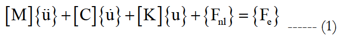
In this equation, [M] is the mass matrix, [C] is the damping matrix [K] is the stiffens linear matrix, {u} is the displacement vector containing the structural Degrees Of Freedom DOF, {Fnl} is a general (nonlinear) restoring function which can depend on the displacements {u}.
Stochastic Perturbation Method
The perturbation method is largely employed in the field of the stochastic finite elements. It is based on an approximation the random variables by their development in Taylor series around their average value. These developments are truncated at the second order. The perturbation method must obey in the conditions of existence and validity, in particular the reduced field of variation of the random variables. We present an extension of this method for the nonlinear dynamic systems with uncertain parameters.
Let us assume that the mass [M], the dumped [C] and the stiffness matrices[K], and The external force vector {Fe}i are related to a vector of the random variables ϑi (i=1,…,I). In the time domain, the stochastic differential system Equation(1) has to be solved. The first two moments of time response (average and variance), will be calculated by using the second order perturbation method.
One defines the vector of the average parameters ϑi− and the quantity dϑi = ϑi - ϑi. All the matrices and vector in Equation (1) are random, and are expanded through second order Taylor series as follows:
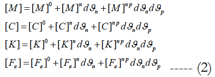
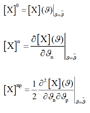
where [.]0, [.]n and [.]np are deterministic matrices corresponding to the zero, the first and the second order partial derivatives with respect to the random parameter ϑi and given by:
Indicial notations are used, with indices n, p running over the sequence 1, 2,…, I as well as the repeated indices summation.
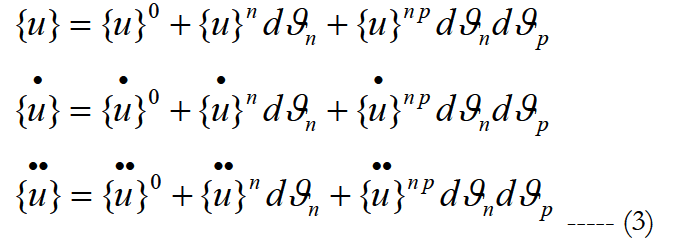
The unknown vectors displacement, velocity and acceleration are also developed through Taylor series as follows:
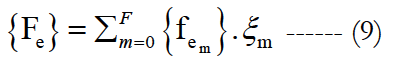
And the vector non linear force:
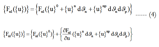
Then
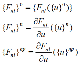
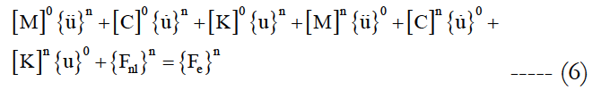
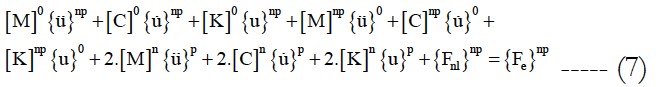
Substituting these developments into Equation (1) and writing the terms of same order on gets the following differential systems:

Polynomial Chaos Expansion Method
The polynomial chaos expansion presented in this section analysis the dynamic behavior of structures with uncertain parameters. the physical properties of structural described by the mass [M], damping [C] and stiffens [K] are random matrices.
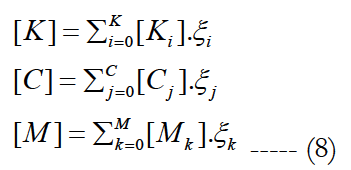
Using a particular formulation of the stochastic finite element method the matrices [M], [C] and [K] can be represented in the form:
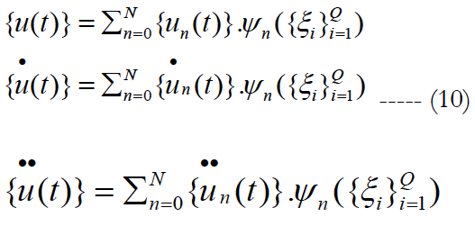
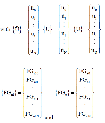
The temporal response of non linear dynamic systems with the random properties is also a random process the vectors u (t), u (t)and u(t) are expanded along polynomial chaos basis.
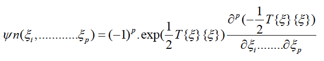
Where ψ(ξi) are multidimensional Hermit orthogonal polynomials in the random variables ξi defined by:
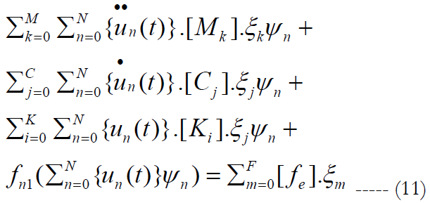
We multiply the equation obtained by ψm. If we used averaged (integration on the domain of random variables), and use the orthogonality properties of polynomials, we obtained the following equation:
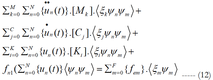
<ξiψn ψm> is the inner product defined by the mathematical expectation operator.
Using matrix notations the resulting algebraic non linear system can be rewritten as:

Note that due to the orthogonality of polynomials, most of expressions <ξiψn ψm> are zero.
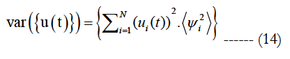
The mean and variance values of {u(t)} are given directly by:
mean({u(t)})={u0(t)}
Stochastic Temporal Response
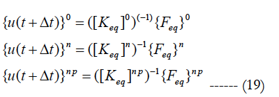
The temporal response from time 0 to time T of equations (5, 6,7 and 13) is required. The time T is subdivided into n intervals Δt = T/n and the numerically solution is obtained at times tr = r.Δt r ∈ IN and 0 ≤ r ≤ n Assuming that the solutions at times t are known and that the solution at time (t + Δt) is required next. According to the Newmark method, the following assumption is used at time (t + Δt):
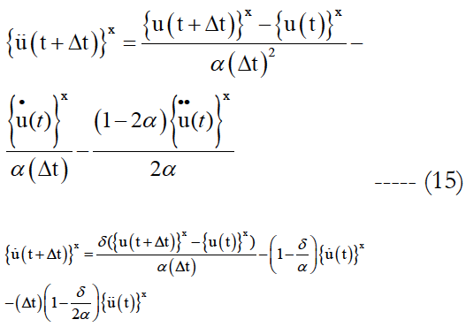
With x can take 0, n, np values.
In which, the two parameters α and δ, verify δ ≥ 1/2 and α ≥ (δ+0.5)/4 in order to get accurate and stable solution. The following notations are used:
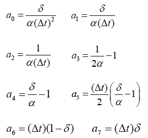
Based on these notations the following equations are resulted.
with:
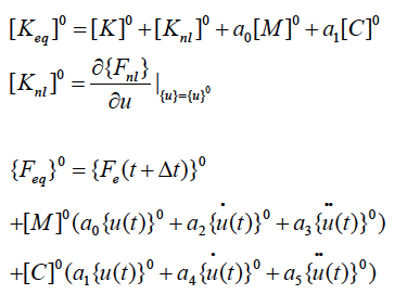
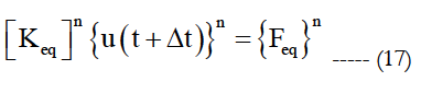
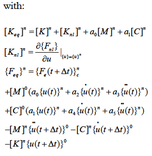
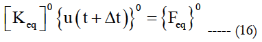
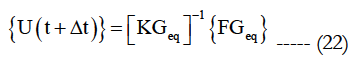
The solution of the problem is obtained by successively solving of the following algebraic equations:
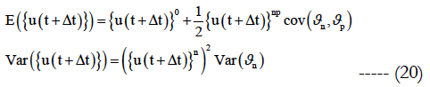
The mean and the variance values of displacement u(t+Δt) are given by:
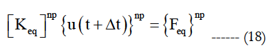
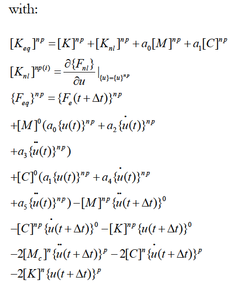
For Polynomial Chaos Expansion Problem
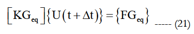
with:
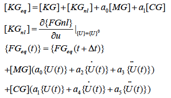
The solution of the problem is obtained by:
With
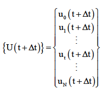
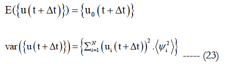
The mean and the variance values of displacement u(t+Δt) are given by:
Numerical Example
For non linear discrete systems with stochastic parameters, some benchmark tests are elaborated to demonstrate the efficiency of the methodological approach. The presented method can be applied to continuous or discrete systems. In this article we restrict ourselves to show the applicability and effectiveness of these methods for the dynamic analysis of nonlinear discrete systems with N DOF. A non linear dynamic system consisting of 20 masses connected by 21 springs nonlinear shown in Figure 1.
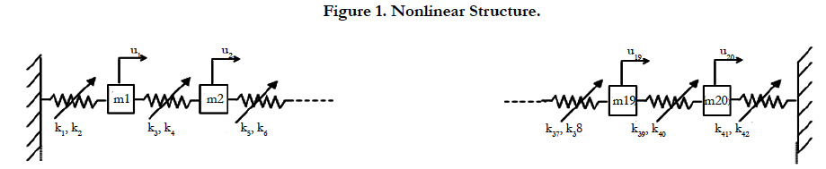
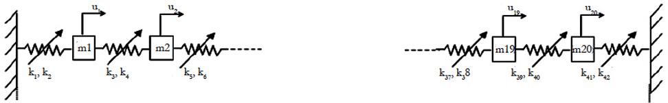
Figure 1. Nonlinear Structure.
The following characteristics are considered:
Masse: m1 = m2 =... = m20 = 2kg
Linear stiffness: k1 = k3 = ...= k39 = k41 = 50N/m;
Non linear cubic stiffness: k2 = k4 ==k42 = 10N/m3
In this study, it has been chosen to investigate the effects of uncertainties by considering different mass uncertain parameters. The mass parameter is supposed to be a random variable and defined as follows: m = m0 (1+σmϑm) Where ϑm is a zero mean value Gaussian random variable, m0 = mi i=1…20 = 2kg is the mean value. ϑm = 2%, ϑm= 5% and ϑm = 7% are the standard deviation of this parameter. Firstly, the mean and variance of the magnitude of displacement have been computed by Polynomial Chaos Expansion, the perturbation method. The obtained results are compared with those given by the direct Monte Carlo simulation 700 simulations. The obtained results are plotted in Figures 2, 3 and 4 which correspond respectively to temporal displacements of the mass m3 for ϑm = 2%, ϑm = 5% and ϑm = 9%. Very small discrepancies between the predictions given by Polynomials Chaos Expansion, perturbation method and Monte Carlo simulation are observed. Again, if more accuracy is needed, then the higher order polynomial chaos can be easily used. In order to highlight the performances of the proposed approach in term of computation cost, the CPU time between the Polynomial Chaos Expansion, perturbation method and Monte Carlo simulation is given in Table 1. A spectacular time reduction is observed when using the Polynomial Chaos Expansion.
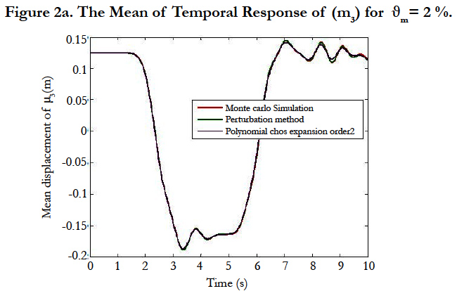
Figure 2a. The Mean of Temporal Response of (m3) for ϑm= 2 %.
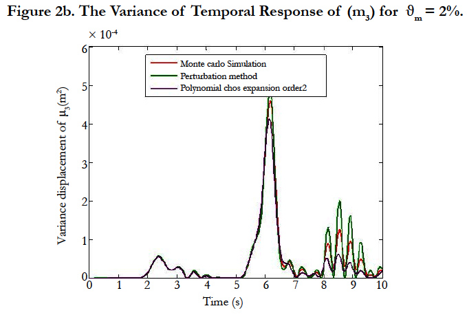

Figure 2b. The Variance of Temporal Response of (m3) for ϑm = 2%.
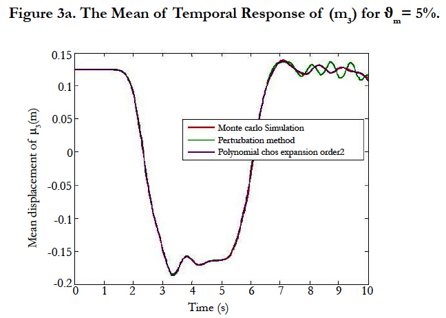
Figure 3a. The Mean of Temporal Response of (m3) for ϑm= 5%.
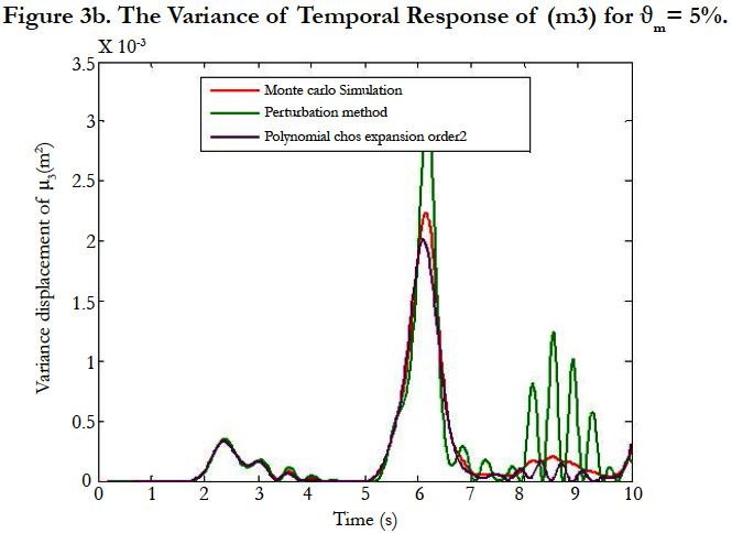
Figure 3b. The Variance of Temporal Response of (m3) for ϑm = 5%.
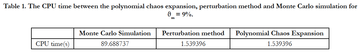

Table 1. The CPU time between the polynomial chaos expansion, perturbation method and Monte Carlo simulation for ϑm = 9%.
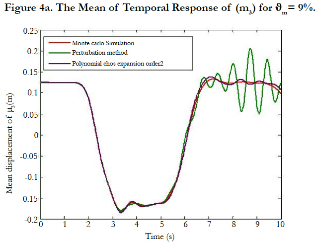
Figure 4a. The Mean of Temporal Response of (m3) for ϑm = 9%.
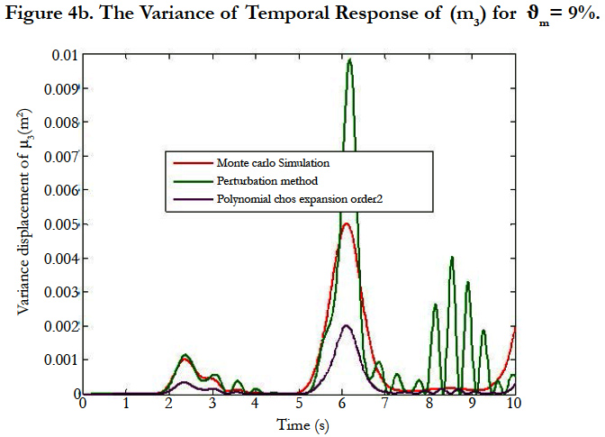
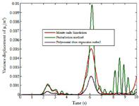
Figure 4b. The Variance of Temporal Response of (m3) for ϑm = 9%.
Conclusion
The main of this work is to provide the variability of the transient solution of a complex structure by considering geometric nonlinearities. We have achieved this by implementing temporal integration for the perturbation method, the polynomial chaos expansion and the Monte Carlo simulation. The perturbation method gives accurate results for low dispersions against when the dispersion increases the polynomial chaos expansion gives good results. The numerical tests show the accuracy of the results and minimization of cost calculation compared to Monte Carlo simulation.
References
- Fishman GS (1996) Monte Carlo: Concepts, algorithms and Applications. (1st Edn), Springer Verlag: Newyork.
- Kleiber M, Hien TD (1992) The stochastic finite element method. Wiley, chichester, UK.
- Zhao L, Chen Q (2000) Neumann dynamic stochastic finite element method of vibration for structures with stochastic parameters to random excitation, Comput Struct. 77: 651-657.
- Muscolino G, Ricciardi G, Impollonia N (1999) Improved dynamic analysis of structures with mechanical uncertainties under deterministic input. PrEM. 15: 199-212.
- R Ghanem (1999) Stochastic finite elements with multiple random nongaussian properties. J Eng Mech. 60(4): 26–40.
- Adhikari S, Manohar CS (1999) Dynamic analysis of framed structures with statistical uncertainties. Int J Numer Method Eng. 44: 1157-1178.
- Li R, Ghanem R (1998) Adaptive polynomial chaos expansions applied to statistics of extremes in nonlinear random vibration. PrEM. 13(2): 125-136.
- Sarsri D, Azrar L (2015) Dynamic analysis of large structures with uncertain parameters based on coupling component mode synthesis and perturbation method. Ain Shams Eng J. 7: 371-381.
- Sarsri D, Azrar L (2016) Time response of structures with uncertain c parameters under stochastic inputs based on coupled polynomial chaos expansion and component mode synthesis methods. Mech Adv Mater Struc. 23(5): 593-606.
- JJ Sinou, J Didier, B Faverjon (2015) Stochastic non-linear response of a flexible rotor with local non-linearities. Int J Non-Linear Mech. 74: 92–99.