Use of the Power of Phase Transition to Explain Turbulence & Sonoluminescence
WS Gan*
Acoustical Technologies Singapore Pte Ltd, Singapore.
*Corresponding Author
WS Gan,
Acoustical Technologies Singapore Pte Ltd, Singapore.
Tel: (65) 90932730
E-mail: wsgan5@gmail.com
Received: October 25, 2016; Accepted: November 28, 2016; Published: December 02, 2016
Citation: WS Gan (2016) Use of the Power of Phase Transition to Explain Turbulence & Sonoluminescence. Int J Aeronautics Aerospace Res, S3:001, 1-8. doi: http://dx.doi.org/10.19070/2470-4415-SI03001
Copyright: WS Gan© 2016. This is an open-access article distributed under the terms of the Creative Commons Attribution License, which permits unrestricted use, distribution and reproduction in any medium, provided the original author and source are credited.
Abstract
First my discovery that every quantum field theory (QFT) problem also has a phase transition solution is described. Examples are given to illustrate this. Then the power of phase transition is used to explain turbulence, sonoluminescence and phase transition also plays a role in the ultimate model of the universe and the unification of the four fundamental forces of nature and the origin of mass in universe. Phase transition solution can also lead to the discovery of new phase of matter, and new material. The status of the phase of a material is above its physical properties. It gives the overall form of the material and the origin of its mass. The explanation of turbulence and sonoluminescence is beyond the limit of fluid mechanics and hydrodynamics. Statistical mechanics and phase transition go to a more fundamental level than fluid mechanics and hydrodynamics in the explananation of turbulence and sonoluminescence. Towards the end of the paper we also give an introduction to the application of the renormalization method to turbulecne as a critical phenomenon and second order phase transition.
2.Introduction
3. Discovery of an Important Theorem of Theoretical Physics
4. Phase Transition – Explanation of Turbulence
5.Phase Transition Explanation of Sonoluminescence
5.1.Experimental confirmation of cooling after bubble collapse down to the critical temperature for light emission
6.Spontaneous Energy Focusing in Sonoluminescence
7.Plasma Formation During Sonoluminescence
8.Turbulence as a Critical Phenomena
9.Application of Renormalization Group Method to Turbulence
10.Conclusion
11.Acknowledgements
8.References
Keywords
Turbulence; Sonoluminescence; Phase Transition; Critical Temperature; Renormalization Group Method.
Introduction
Second order phase transition and spontaneous symmetry breaking (SSB) were pioneered by L Landau [1] in 1937 and plays a key role in the origin of the universe as demonstrated by the origin of mass played by the Higgs boson [2] as a second order phase transition and subsequent formation and decay of particles after the BIG BANG are symmetry breaking phase transitions. Phase transition also plays a role in condensed matter physics as shown by the combination of the fields solid state physics and liquid state physics into a single field of condensed matter physics due to the role of condensation and phase transition. In this paper we will use the power of phase transition to explain turbulence and sonoluminescence and show that phase transition also plays a key role in the ultimate model of the universe. But I will start with my recent discovery that every quantum field theory (QFT) problem also has a phase transition solution. Phase transition and statistical mechanics enable a more fundamental understanding of these two phenomena. We started using Landau [1]’s second order phase transition. Since phenomenology, it cannot explain the region around the critical temperature. We made a preliminary application of Ken Wilson [3]’s renormalization group method to turbulence and sonolumniescence which are both critical phenomena and second order phase transition.
Discovery of an Important Theorem of Theoretical Physics
Recently I discovered an important theorem in theoretical physics that every quantum field theory (QFT) problem also has a phase transition solution. This was inspired by my own PhD (1969) thesis [4] in which I pioneered the use of statistical mechanics approach to ultrasound propagation in semiconductor in the presence of high magnetic fields and low temperatures. The usual method is electron-phonon interaction of many body theory of QFT. In my thesis the Boltzmann transport equation, an important equation in non-equilibrium statistical mechanics is used. In this problem the phase transition is from metal to semiconductor and it is beyond the limit of many body theory. For metals, electrons move freely and free electron model is sufficient. In semiconductor, there is attraction between electrons The problem is too complex to be handled by many body theory alone and it is beyond the limit of QFT. A beautiful example of this characteristics is the BCS theory of superconductivity [5] which has QFT solution of many body theory of electron-electron interaction and Coopers pairing as well as the second order phase transition solution from metal to superconductivity with spontaneous symmetry breaking (SSB). Since the mid 1960s, the name of solid state physics has been changed to condensed matter physics to reflect the important role played by statistical mechanics and phase transition besides QFT. Thus my PhD (1969) [4] thesis played a role in the founding of the field of condensed matter physics. Nowadays in the American Physical Society, condensed matter physics group has the largest number of members. This shows the importance of the field.
This important discovery also shows that Yang Mills theory [6] is only a partial solution of the theory of the Standard Model. It describes correctly the various forces and interaction between the particles. Higgs theory [2] which is phase transition solution is required to explain the origin of mass. Thus a complete theory of the standard model has two parts, the QFT solution and the phase transition solution.
Another illustration is before the 1960s, there were the separate fields of solid state physics and liquid state physics and the only theoretical framework is many body theory of QFT. With the discovery of Bose Einstein condensate, the two fields combined to form the new field of condensed matter physics which shows the role played by phase transition solution. In fact, phase solution and statistical mechanics is required for liquid state physics as it is beyond the limit of QFT.
There are also two other classic examples to illustrate this important discovery. One is Nambu [7]’s introduction of second order phase transition from condensed matter physics into QFT to explain the broken local gauge invariance when mass is introduced into the Yang Mills [6] theory. This confirms that phase transition is another part of the solution of the Standard Model. Another classic example is that of Kenneth Wilson [3]’s introduction of the renomalization group from statistical mechanics and phase transition into QFT to solve the renormalization problem in quantum chromodynamics (QCD). He introduced the lattice version or discrete version of QCD in oppose to the continuum formulation of the theory. This idea is originated from his prior works in statistical mechanics. This again confirms that phase transition solution (statistical mechanics) is another part of the solution of QFT. It is of interest to note that Nambu [7] and Higgs [2] introduced SSB into particle physics but never mentioned ‘phase transition’ in their papers although second order phase transition involves SSB. This is because their focus is on the QFT solution and not the phase transition solution.
This discovery of the characteristics of a QFT problem is useful as a guide in solving QFT problem just like symmetry can be used as guide in solving complex physics equations as every fundamental law of physics has symmetry properties as mentioned by Richard Feymann [8]. The role of phase transition is very important because it can lead to discovery of new material compared with QFT which only describes what is happening within the material. An example is the discovery of the topological insulators and superconductors from topological phase transition by Xiao-Liang Qi and Shou-Cheng Zhang [9] in 2010. The creation and the formation of matter has to do with phase transition. That is why phase transition is responsible for the creation of the universe, for the creation of the BIG BANG and the black hole and the origin of mass.
Phase Transition – Explanation of Turbulence
Turbulence is an important topic in nonlinear acoustics which is still not properly explained. The major breakthrough was the work of Kolmogorov [10] in 1941 who is the first to introduce the statistical theory of turbulence, resulting in the concept of turbulence as an inverse cascade. Turbulence is a very complex phenomenon and sofar we are unable to explain what is inside turbulence. Most of the works done on turbulence are of fluid mechanics or hydrodynamics in nature. To explain turbulence, one has to go beyond the limit of fluid mechanics to statistical mechanics and phase transition.
I introduce field theory into turbulence. Kolmogorov [10]’s work shows the statistical properties of the turbulence field. The field theory approach will also pave the way for the application of quantum field theory to turbulence below. Now there is a trend of moving towards second order phase transition and statistical mechanics to interpret turbulence. In 2009 W S Gan [11] proposed turbulence as a second order phase transition with SSB. Examples of second order phase transition with SSB are magnetization, superconductivity and superfluidity, topics in condensed matter physics. Hence turbulence is also a field in condensed matter physics. My hypothesis has been subsequently supported by the works on Nigel Goldenfeld [12]'s group which showed that turbulence has the same behavior as magnetization. In his paper, he presented experimental evidence that turbulence flows are closely analogous to critical phenomena from a reanalysis of friction factor measurements in rough pipes. He found experimentally two aspects that confirm that turbulence is similar to second order phase transition such as magnetization in a ferromagnet. These are experimentally verified power law scaling of correlation function which is remininescent of the power law fluctuations on many length scales that accompany critical phenomena for example in a ferromagnet near its critical point which is second order phase transition. Another aspect is the phenomena of data collapse or Widom scaling [13]. For example, in a ferromagnet, the equation of state, nominally a function of two variables is expressible in terms of a single reduced variable which depends on a combination of external field and temperature. This has been confirmed by the experiments of J Nikuradze [14] in 1932 and 1933 which showed data collapse. Goldenfeld [12]’s work proposed that the feature of the turbulence can be understood as arising from a singularity at infinite Reynolds number and zero roughness. Such singularities are known to arise as second order phase transition such as that occurs when iron is cooled down below the Curie temperature and becomes magnetic. The theory predicts that the small scale fluctuation in the fluid speed, a characteristic of turbulence e connected to the friction and can be demonstrated by plotting the data in a special way that causes all of the Nijkuradze [14] curves at different roughness to collapse into a single curve. According to Goldenfeld [12]’s study, the formation of eddies in turbulence might be a similar phenomenon to the lining of spins in magnetization. Eddies are thus similar to the clusters of atoms. Goldenfeld et al., [12] hope that as a result of these discoveries, the approaches that solved the problem of phase transitions will now find a new and unexpected application in providing a fundamental understanding of turbulence. In 2013, W. S. Gan [15] extended L Landau [1]’s theory of second order phase transition from phenomenology to a more rigorous approach by using statistical mechanics and gauge theory. We propose turbulence as a classical analog of Bose Einstein condensation and the Gross- Pitaevskii equation is used to derive the condensate free energy. The critical value of the order parameter, the condensation wave function is determined. This is the value when turbulence occurs and SSB in the ground state of the condensation free energy takes place. Being a condensate, there is molecular pairing in turbulence. We determine the numerical value of the condensate free energy with the use of the coupled oscillation model for the pair of molecules. Our expression for the condensation free energy also yields a power series in terms of the order parameter in agreement with the Landau phenomenology of second order phase transition. This confirms that turbulence is a condensate, since Gross-Pitaevskii equation is the equation for condensate. We conclude that our understanding of turbulence is a second order phase transition and is a condensate with molecular pairing.
Kolmogoro [10]’s theory is based on scale invariance and selfsimilarity and Ken Wilson [7]’s application to critical phenomena and second order phase transition is also based on scale invariance. Kolmogorov [10]’s theory is calculation of energies of different length scales and Ken Wilson [7]’s renormalization group application to critical phenomena is also calculation of energies of different length scales. So it is natural to extend Kolmogorov [10]’s scaling invariance to renormalization group treatment of turbulence. The renormalization group treatment of turbulence is more sophisticated than Kolmogorov [10]’s scaling law treatment. Ken Wilson [7]’s papers on the application of renormalization group to critical phenomena and second order phase transition confirmed that turbulence is a critical phenomena and second order phase transition.
In hydrodynamics, the atomic fluctuations averaged out and classical hydrodynamics equations like Navier-Stokes equations emerged and this is continuum treatment. Unfortunately there is much more difficult class of problems that fluctuations persisted out to a microscopic measurement and fluctuations on all intermediate length scales are important too. Examples are fully developed turbulence flow, critical phenomena and elementary particles physics. This again confirms that turbulence has feature of critical phenomena.
Turbulence is the case where microscopic fluctuations remain even to macroscopic wavelength. In fully developed turbulence in atmosphere, global air circulation becomes unstable leading to eddies on a scale of thousands of miles. These eddies break down into small eddies, which in turn break down until chaotic motions in all length scales down to millimetres have been excited. On the scales of millimetres, viscosity damps the turbulence fluctuations and no small scales are important until atomic scales are reached. Renormalization group (RG) approach is strategy for dealing with problems involving many length scales like turbulence. The strategy is to tackle the problems in steps, one step for each scale. In the case of critical phenomena, the problem technically is to carry out statistical averages over thermal fluctuations on all size scales. The RG approach is to integrate out the fluctuations in sequence starting with fluctuations on an atomic scale then moving to successively larger scales until fluctuations on all scales have been averaged out.
The Landau [1] theory has the same physical motivation as hydrodynamics. Landau [1] assumes that only fluctuations on an atomic scale matters . In order to study the effects of fluctuations only a single wavelength scale will be considered. This is the basic step in RG. In theoretical physics, the RG refers to a mathematical apparatus that allows systematic investigation of the changes of a physical system as viewed at different distance scales. In particle physics, it reflects the changes in the underlying force laws modified in a quantum field theory (QFT) as the energy scale at which physical processes occur varies, energy/momenta and resolution distance scales being effectively conjugate under the uncertainty principle (cf Compton wavelength). A change in scale is called a scale transformation. The RG is intimately related to scale invariance & conformal invariance, symmetries in which a system appears the same at all scales(so called self-similarity). This property of turbulence field is also used in Kolmogorov [10]’ scale invariance treatment of turbulence. This also confirms that the turbulence field has both statistical and symmetries property. In Ken Wilson’s Nobel Lecture [7], he mentioned that fully developed turbulence has a critical point which is a feature of critical phenomena. Landau [1]’s theory of second order phase transition is a phenomenology and a mean field theory. It failed in the behaviour of the region surrounding the critical point or the critical temperature. The RG method will improve on this. Only the effects of wavelengths long compared to atomic scales will be discussed and it will be assumed that only modest correction to the Landau [1] theory are required.
To extend the renormalization group method to turbulence, one has to introduce the fluctuation of length scale into the Landau- Ginzburg integral of free energy:
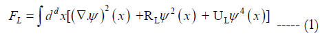
where Ψ = condensation wave function = order parameter, R,U = constants and are functions of temperature T, d = dimension and L = length somewhat larger than atomic dimension.
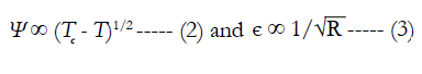
Here we treat turbulence as a Bose-Einstein condensate. The RG method treatment of the critical point is an improvement over the Landau ‘s phenomenology of second order phase transition which failed at the region near the critical point or critical temperature where the second order phase transition takes place. This is because Landau ignores the persistent intermediate length scale and treat it as the averaging out as the atomic length scale which amounts to a continuum which is not the case.
The importance of long wavelength fluctuation means that the parameters R and U are dependent on L. The L dependence persists only out to the correlation length є. Fluctuations with wavelength >є will be seen to be negligible. Once all wavelengths of fluctuations out to L ~є have been integrated out, one can use the Landau theory. This means that we can substitute in R< ε and in Uε the following equations:
In order to study the effects of fluctuations, only a single wavelength scale will be considered. To be precise, consider only fluctuation with wavelengths lying in an infinitesimal interval L to L + δL. As the fluctuation on each length scale are integrated out a new free energy functional FL+δL is generated from the previous functional FL. This process is repeated many times. If FL and FL+δL are expressed in dimensionless form, then one finds that the transformation leading from FL to FL+δ is repeated in identical form many times. The transformation group thus generated is called the renormalization group. As L becomes large the free energy FL approaches a fixed point of the transformation and thereby becomes independent of details of the system at the atomic level. This leads to an explanation of the universality of critical behavior for different kinds of systems at the atomic level. The principal critical point is characterized by two parameters: the dimension d and the the number of internal components n. Great efforts were made to map out critical behavior as functions of d and n. A serious problem in the renormalization group transformation (real space or otherwise) is that there is no guarantee that they will exhibit fixed points. For some renormalization group transformations, iteration of a critical point does not lead to a fixed point presumably field interactions with increasingly long range forces.
Phase transition is another example of the theorem that every QFT problem also has a phase transition solution. The phase transition part is the interaction between the molecules and the phase transition solution is the second order phase transition from the laminar flow phase to the turbulence flow phase.
Phase Transition Explanation of Sonoluminescence
Sonoluminescence was discovered in France in 1933 [16] but sofar it has not been properly explained. Sonoluminescence is another example that it has both a QFT solution and a phase transition solution. The usual explanation of the light emission is the QFT solution as it describes the molecular interaction in chemistry using quantum mechanics which is known as chemiluminescence. To have a complete solution for the explanation of sonoluminescence, the phase transition from the heat energy phase to the light energy phase has to be added.
During the last fifteen years, there is a trend towards the application of statistical mechanics and phase transition explanation of sonoluminescence. Before that, the usual explanation is based on hydrodynamics and the use of Navier Stokes equation. This can only describe the phenomenon without explaining the root of the problem which is beyond the capability of hydrodynamics. It also shows the application of the theorem that every QFT problem also has a phase transition solution. The QFT problem is the interaction among the molecules and the phase solution is the conversion from the heat phase to the light phase.
Sonoluminescence can be interpreted as a two stages process. The first stage happens when the bubble collapses with broken spherical symmetry. Tremendous heat is released with temperatures reaching 20,000 kelvin. This part of the theory has been described in details by D F Gaitan et al., [17] The second stage is the cooling down of the system with subsequent light emission. The description has been by K S Suslick et al., [18]. Our work here will focus on the second stage of the process, on the phase transition solution as the QFT solution using quantum mechanics to describe light emission due to molecular interaction has been done by several authors.
Second order phase transition with SSB in statistical physics was pioneered by L Landau [1]. Here we describe sonoluminescence as a Bose Einstein condensate and the following Gross-Pitaevskii equation is used:
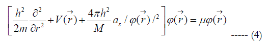
where M = mass of the boson, V = external potential, as = bosonboson scattering length, μ = chemical potential & ћ = retarded Planck’s constant.
The Landau order parameter here is the condensation wave function. The Gross-Pitaevskii equation describes the ground state of a quantum system of identical bosons using the Hartree-Fock approximation and the potential interaction model.
In the Hartree-Fock approximation, the total wave function φ of the system of N bosons is taken as a product of single, particle function φ:
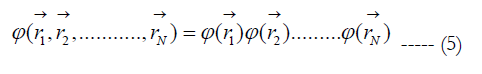
The pseudopotential model Hamiltonian of the system is given as:
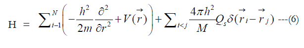
where δ (r )→is the Dirac delta function. (4) is the model equation for the single particle wave function in a Bose-Einstein condensate. It is similar in form to the Ginzburg-Landau equation. Since light emission occurs after temperature cools down or condenses after the tremendous heat emission after bubble collapse, sonoluminescence can be interpreted as a Bose Einstein condensate and hence the Gross-Pitaevskii equation is used.
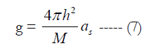
A Bose Einstein condensate is a gas of bosons that are in the same quantum state and thus can be described by the same wave function. A free quantum particle is described by a single-particle Schrondinger equation. Interaction between particles in a real gas is taken into account by pertinent many body Schrodinger equation. If the average spacing between the particles in a gas is greater than the scattering length, then one can approximate the true interaction potential that features in this equation by a pseudopotential. The nonlinearity of the Gross-Pitaevskii equation has its origin in the interaction between the particles. This becomes evident by equating the coupling constant of interaction in the Gross-Pitaevskii equation with zero on which the single particle Schrondinger equation describing a particle inside a trapping potential is recovered. Then the equation has the form of Schrondinger equation with the addition of an interaction term. The couping constant g is proportional to the scattering length of two interacting bosons:
The energy density is:
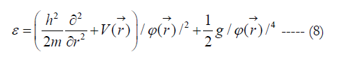
where φ = condensation wave function, = Landau order parameter and V = external potential.
The condensation free energy Δε is given by the difference between the light and heat state free energy. From (8), the light state free energy is given by:
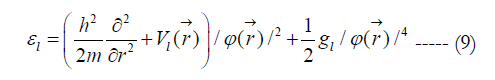
The heat state free energy is given by:
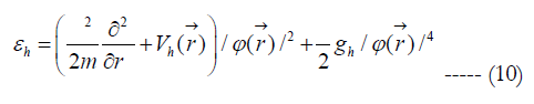
Where + 1/2 g/φ (r→)4 is the nonlinear interaction term.
We consider that the light emission is due to nonlinear interaction between the molecules and the mechanism of the interaction is the pairing of the water molecules, a special case of nonlinear interaction. This is the quantum field theory solution of sonoluminescence. The pairing of water molecules gives rise to light emission and this is the origin of sonoluminescence. The condensation free energy is given by:
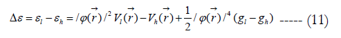
This will be the ground state of the Hamiltonian of light emission free energy. The critical value of the order parameter is corresponding to that for minimum condensation free energy and this is when light emission occurs. There is also spontaneous symmetry breaking (SSB) at the ground state giving rise to second order phase transition and light emission. The critical values of SSB can be obtained as follows:
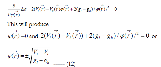
The meaning of ϕ(r)→ = 0 means that there is only one value for the order parameter and there is no broken symmetry [12]. shows that there are two values of the order parameter or condensation wave function when light emission occurs or when there is a degeneracy of the ground state of the Hamiltonian. This confirms spontaneous symmetry breaking in the ground state of the condensation free energy when light emission occurs.
The phenomenon of sonoluminescence is primarily of thermal origin, i.e. caused by high temperatures rather than high pressure or densities. The determination of the minimum temperature required of light emission is therefore important in understanding the mechanism involved. According to the theories, the minimum temperature necessary to generate observables sonoluminescence is between 2000 and 3000K corresponding to relative densities of 100-200. Suslick et al [18] measured a temperature of 5200 ± 650K inside cavitation bubbles. This confirms that indeed the system cools down after bubble collapse to reach the critical temperature of 2000 to 3000 K for light emission and that there is a second order phase transition after the bubble collapse to produce light emission.
The internal temperature measured in Suslick et al.,[18]’s experiments indicate that present theories of bubble pulsation may overestimate the internal temperature and possibly the internal pressure too. The over estimation may be explained by the failure of the assumptions made in the models. Specifically the dissociation of the gas molecules due to the high temperature attend will increase the number density and therefore the internal gas pressure, resulting the bubble collapse sooner than predicted. When temperatures of 5000K or higher are reached, it is likely that the energy of the collapse is partitioned into other chemical processes, instead of increasing the temperature of the gas. Some of these processes include dissociation of the gas molecules and ionization. Thus, as the strength of the collapse increases, i.e. at larger value of pressure, the internal temperature is expected to reach a plateau. In addition, the models underestimate the effects of energy dissipation due to the compressibility of the liquid. A compressible liquid results in the formation of shock wave that may cause a significant portion of the collapse energy away from the bubble.
Spontaneous Energy Focusing in Sonoluminescence
There is spontaneous energy focusing in sonoluminescence Low amplitude sound energy entering a fluid spontaneously focuses by 12 orders of magnitude to create a flash of light and a new phase of matter. The energy Poynting vectors of the molecules all focus in one direction in space, causing the system to break the rotational invariance of the Hamiltonian spontaneously. This confirms that sonoluminescence is a second order phase transition.
Plasma Formation During Sonoluminescence
Also plasma formation has been observed during sonoluminescence [19]. Plasma is the fourth state of matter. This confirms that sonoluminescence is phase transition.
Thus phase transition provides the big picture of sonoluminescence with the gaps in the details to be further investigated.
Turbulence as a Critical Phenomena
Ken Wilson [3] Nobel lecture described turbulence as a critical phenomena. Since critical phenomena, it is also a second order phase transition. There are a lot of complex problems in science, when complex microscopic behaviour unlies macroscopic effects. In simple cases, the microscopic fluctuations average out when larger scales are considered and the averaged quantities satisfy classical continuum equations. Hydrodynamics is a standard example of this where atomic fluctuations averaged out and the classical hydrodynamic equations emerge. Unfortunately there is a much more difficult class of problems where fluctuations persist out to macroscopic wavelength and fluctuations on all intermediate length scales are important too. Fully developed turbulence is an example of the last category.
In fully developed turbulence in the atmosphere, global air circulation becomes unstable, leading to eddies on a scale of thousands of miles. These eddies break down into smaller eddies which in turn break down until chaotic motion on all length scales down to millimetres have been excited. On the scale of millimetres, viscosity damps the turbulence fluctuations and no smaller scales are important until atomic scales are reached. A critical point is a special example of a phase transition. It takes many variables to characterize a turbulent flow near the critical point.
The renormalization group approach is a strategy for dealing with problems involving many length scales. The strategy is to tackle the problem in steps, one step for each length scale. In the case of critical phenomena, renormalization group is an improvement to Ginzburg-Landau [1] theory. The problem technically is to carry out statistical average over thermal fluctuations on all size scales. The renormalization group approach is to integrate out the fluctuations in sequence starting with fluctuations on an atomic scale until fluctuations on all scales have averaged out . The renormalization group method is an improvement to Ginzburg-Landau [1] theory.
The renormalization group method that was defined in 1971 by Ken Wilson [3] embraces both practical approximations leading to actual computation and a formalism. Here the central idea of fixed point is illustrated. As the fluctuations on each length scale are integrated out a new free energy functional FL+δL is generated from the previous functional FL, This process is repeated many times. If FL and FL+δL are expressed in dimensionless forms then one finds that the transformation leading from FL to FL+δL is repeated in identical forms many times . The transformation group then generated is called the renormalization group. As L becomes large the free energy FL approaches a fixed point of the transformation and thereby becomes independent of the details of the system at the atomic level. This leads to an explanation of the universality of critical behaviour for different kinds of systems at the atomic level.
Application of Renormalization Group Method to Turbulence
To demonstrate the fixed point form of the free energy functional, it must be put into dimensionless form. Lengths need to be expressed in units of L and and rewritten in dimensionless forms. The Ginzburg-Landau [1] free energy is given as :
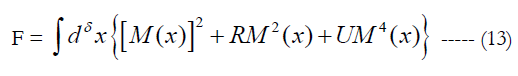
where R,U = temperature dependent constants, M = Landau order parameter.
We shall assume Ginzburg-Landau [1] analysis is valid for the form of F. For long wavelength fluctuations mean that the parameters R and U depend on L. Thus F should be denoted FL:
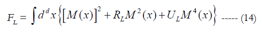
The breakdown of analyticity at the critical point or critical temperature is a simple consequence of this L dependence. The L dependence persists only out to the correlation length ξ: fluctuations with wavelength >ξ will be seen to be always negligible. Once all wavelengths of fluctuations out to L~ξ have been integrated out, one can use the Ginzburg-Landau- [3] theory. Since ξ is itself non-analytic in T at T= Tc the dependence of Rξ and Uξ on ξ introduces new complexities at the critical point.
In a world with greater than four dimensions, the Ginzburg-Landau [3] picture is correct. Four dimensions is the dividing line, -below four dimensions, fluctuations on all scales up to the correlation length are important and Ginzburg-Landau [1] theory breaks down. The role of long wavelength fluctuations is very much easier to work out near four dimensions where their effects are small. So this is the only case that will be discussed here. Only the effects of wavelengths long compared to atomic scales will be discussed and it will be assumed that only modest corrections to the Ginzburg-Landau [1] theory are required.
For d<4 and sufficiently large L, Ken Wilson [3] has obtained:
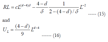
The above equations (13) to (16) are valid for all Bose Einstein condensates. They are applied here to turbulence which also has the above scale invariance properties but with its own characteristic of L and correlation length.
First the Richardson [20]’s cascade picture of turbulence known as the energy cascade:
1. A turbulent flow is composed by eddies of different sizes,
2. The large eddies are unstable and eventually breaks up into smaller eddies and so on,
3. The energy is passed down from the large scales of motion to smaller scales until reaching a sufficiently small length scales such that the viscosity of the fluid can effectively dissipate the kinetic energy.
The energy cascade is described as a breakdown process of eddies into smaller eddies which fill a lesser portion of space with a spatial distribution prescribed by the model.
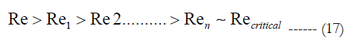
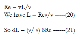
The modern concept of fully developed hydrodynamic turbulence is based on Richardson [20]’s cascade model for Re = vL/ν >>1 where Re = Reynolds number, ν = viscosity, v = velocity flow and L = size of a streamlined body = characteristic scale of the velocity field:
.PNG)
This cascade of decays goes on until the Reynolds number calculated with the help of the size and the velocity of nth generation eddies is about some Recritical :
The last generation eddies are stable and they dissipate due to viscosity . At the critical value of the Reynolds number, L is given by
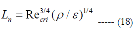
where ρ = density of fluid.
Kolmogorov [10]'s second hypothesis states that for very high Reynolds numbers the statistics of small scales are universally and uniquely determined by the kinematic viscosity ν and the rate of energy dissipation ε. With only these two parameters, the unique length that can be formed by dimension analysis is:

where η = Kolmogorov’s length scale, ν = kinematic viscosity, and ε = rate of energy dissipation.
A turbulent flow is characterized by a hierarchy of scales through which the energy cascade takes place. Dissipation of kinetic energy takes place at scales of the order of Kolmogorov length(Kolmogorov microscales) η, while the input of energy into the cascade comes from the decay of the large scales, of order L. These two scales at the extremes of the cascade can differ by several orders of magnitude at high Reynolds numbers. In between there is a range of scales(each one with its own characteristic length r) that has formed at the expense of the energy of the large ones. These scales are very large compared with the Kolmogorov length, but still very small compared with the large scale of the flow(i.e. η << r << L). Since eddies in this range are much larger than the dissipative eddies that exist at Kolmogorov scales, kinetic energy is essentially not dissipated in this range, and its is merely transferred to smaller scales until viscous effects become important as the order of the Kolmogorov scale is approached. Within this range inertial effects are still much larger than viscous effects, and it is possible to assume that viscosity does not play a role in their internal dynamics (for this reason this range is called inertial range).
Here we replace the L in eqns (15) and (16) by the Kolmogorov length η. From the equation for the Reynolds number:
The δL in the free energy functional FL+δL will be replaced by the δL in eqn.(9). This will enable the iteration work from FL to FL+δL to obtain the fixed point or the critical point/critical temperature.
Ken Wilson [3] has derived a relation between the critical temperature where phase transition temperature takes place and the correlation length as:
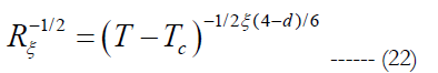
where ξ = correlation length.
Conclusion
My discovery that every QFT problem also has a phase transition solution shows the power of phase transition. It is responsible for the creation and formation of matter, including the creation of the universe, the BIG BANG, the black hole, the creation and the decay of particles. Phase transition goes beyond the Standard Model. It gives the big picture of the ultimate model of the universe with details of interaction and forces between the particles, including the dark energy and dark matter particles to be given by QFT solutions such as the supersymmetry. Phase transition can be used to give a better explanation for turbulence and sonoluminescence. The renormalization group(RG) method is applied to turbulence as turbulence is a critical phenomena and second order phase transition. This is a correction to the Ginzburg-Landau theory of second order phase transition which is phenomenology and a mean-field theory and unable to describe the region near the critical point or critical temperature correctly. This is process of iteration to reach the fixed point or critical point. We have laid down the equations and the algorithms for this work. Phase transition can also lead to the discoveries of new phase of matter and new materials. It even plays a role in the grand unification of the four fundamental forces of nature. This is another example of unification of four forces of nature being a quantum field theory problem also has a phase transition solution.
Acknowledgements
The author wishes to thank the management of Acoustical Technologies Singapore Pte Ltd for permission to publish this work.
References
- L Landau (1937) On The Theory Of Phase Transitions. Theory Of Phase Transitions. 7: 19–32.
- PW Higgs (1964) Broken Symmetries and the Masses of Gauge Bosons.Phys Rev Letts. 13(16): 508-509.
- KG Wilson (1971) Renormalization Group and Critical Phenomena. I. Renormalization Group and the Kadanoff Scaling Picture. Phy Rev B. 4(9): 3174- 3183.
- Gan WS (1969) PhD thesis, Imperial College London, To be published.
- J Bardeen, LN Cooper, JR Schrieffer (1957) Theory of Superconductivity. Phy Rev. 108(5): 1175.
- CN Yang, RL Mills (1954) Conservation of Isotopic Spin and Isotopic Gauge Invariance. Phys Rev. 96(1): 191-195.
- Y Nambu, G Jona- Lasinio (1960) Dynamical Model of Elementary Particles Based on an Analogy with Superconductivity. presented at the Midwestern Conference on Theoretical Physics. Phys Rev. 122(1): 345-358.
- R Feynman (1965) The character of Physical law. BBC. 1-176.
- XL Qi, SC Zhang (2011) Topological insulators and superconductors. Rev Mod Phys. 83: 1057-1110.
- AN Kolmogorov (1941) The Local Structure of Turbulence in Incompressible Viscous Fluid for Very Large Reynolds' Numbers. Doklady Akad Nauk SSSR. 30: 301-305.
- Gan WS (2009) Proceedings of ICSV16, Krakow, Poland.
- N Goldenfeld (2006) Roughness-Induced Critical Phenomena in a Turbulent Flow. Phys Rev Lett. 96: 044503.
- B Widom (1965) Equation of state in the Neighborhood of the critical point. J Chem Phys. 43: 3898-3905.
- J Nikuradse (1933) Technical Memorandum 1292. National Advisory Committee For Aeronautics. 361.
- WS Gan (2013) Towards the Understanding of Turbulence. JBAP. 2(5): 1-9.
- N Marinesco, JJ Trillat (1933) Action des ultrasons sur les Plaques photographiques. J CR Acad Sci. Paris. 858.
- Gaitan DF, Crum LA, Church CC, Roy RA (1992) Sonoluminescence and bubble dynamics for a single, stable, cavitation bubble. J Acoust Soc Am. 91: 3166-3183.
- Suslick KS, Hammerton DA, Cline RE (1986) The sonochemical hot spot. J Am Chem Soc. 108(18): 5641-5642.
- Suslick KS, Flannigan DJ (2009) Plasma conditions during single bubble sonoluminescence. paper presented at the 158th Meeting of the Acoustical Society of America. 126: 2240.
- Richardson, Lewis Fry (1922) Weather Prediction by Numerical Processes. Cambridge University Press, India.