Failure-Oriented-Accelerated-Testing And Its Role In Assuring Reliability Of Aerospace Electronics
E. Suhir*
Bell Laboratories, Murray Hill, NJ (ret), Portland State University, Portland, OR, and ERS Co., Los Altos, CA, 94024, USA.
*Corresponding Author
E. Suhir,
Bell Laboratories, Murray Hill, NJ (ret), Portland State University, Portland, OR, and ERS Co., Los Altos, CA, 94024, USA.
Tel: 650-969-1530
Email: suhire@aol.com
Received: November 11, 2022; Accepted: December 02, 2022; Published: December 05, 2022
Citation:E. Suhir. Failure-Oriented-Accelerated-Testing And Its Role In Assuring Reliability Of Aerospace Electronics. Int J Aeronautics Aerospace Res. 2022;09(2):274-290.
Copyright: E. Suhir© 2022. This is an open-access article distributed under the terms of the Creative Commons Attribution License, which permits unrestricted use, distribution and reproduction in any medium, provided the original author and source are credited.
Abstract
An highly focused and highly cost effective failure-oriented-accelerated-testing (FOAT) suggested about a decade ago as
an experimental basis of the novel probabilistic design for reliability (PDfR) concept is intended to be carried out at the
design stage of a new electronic packaging technology and when high operational reliability (like the one required, e.g., for
aerospace, military, or long-haul communication applications) is a must. On the other hand, burn-in-testing (BIT) that is
routinely conducted at the manufacturing stage of almost every IC product is also of a FOAT type: it is aimed at eliminating
the infant mortality portion (IMP) of the bathtub curve (BTC) by getting rid of the low reliability "freaks" prior to shipping
the “healthy” products, i.e., those that survived BIT, to the customer(s).When FOAT is conducted, a physically meaningful
constitutive equation, such as the multi-parametric Boltzmann-Arrhenius-Zhurkov (BAZ) model, should be employed to
predict, from the FOAT data, the probability of failure and the corresponding useful lifetime of the product in the field,
and, from the BIT data, as has been recently demonstrated, - the adequate level and duration of the applied stressors, as well
as the (low, of course) activation energies of the "freaks". Both types of FOAT are addressed in this review using analytical
("mathematical") predictive modeling, as well as FOAT carried out at the electronic product development stage. The general
concepts are illustrated by numerical examples. It is concluded that predictive modeling should always be conducted prior
to and during the actual testing and that analytical modeling should always complement computer simulations. Future work
should be focused on the experimental verification of the obtained findings and recommendations.
2.Introduction
3.Literature Review
4.Dimensional analysis and Similitude
5.Design procedure of gating and runners
6.Experimental Procedures
7. Conclusion
8. References
Keywords
Accelerated Life Testing (ALT); Bathtub Curve(BTC); Boltzmann-Arrhenius-Zhurkov (BAZ) Equation;
Burn-In-Testing (BIT); Failure-Oriented-Accelerated-Testing (FOAT); Highly Accelerated Life Testing (HALT); Infantmortality-
Portion (IMP); Probabilistic Design for Reliability (PDfR).
Background/Incentive
The bottleneck of an electronic, photonic, MEMS or MOEMS
(optical MEMS) system's reliability is, as is known, the mechanical
("physical") performance of its materials and structural elements
[1-5] and not its functional (electrical or optical) performance,
as long as it is not affected by the mechanical behavior of the
design. It is well known also that it is the packaging technology
that is the most critical undertaking, when making a viable, properly
protected and effectively-interconnected electrical or optical
device and package into a reliable product. Accelerated life testing
(ALT) [6-15] conducted at different stages of an IC package
design and manufacturing is the major means for achieving
that. Burn-in-testing (BIT) [16-23], the chronologically final ALT,
aimed at eliminating the infant mortality portion (IMP) of the
bathtub curve (BTC) prior to shipping to the customer(s) the
"healthy" products, i.e. those that survived BIT, is particularly important:
BIT is therefore an accepted practice for detecting and
eliminating possible early failures in the just fabricated products
and is conducted at the manufacturing stage of the product fabrication.
Original BITs used, as is known, continuously powering
the manufactured products by applying elevated temperature
to accelerate their aging, but today various stressors, other-thanelevated-
temperature, are employed in this capacity. BIT, as far
as "freaks" are concerned, is and always has been, of course, a
FOAT type of testing.
But there is also another, so far less well-known and not always
conducted today, FOAT [24-29] that has been recently suggested
in connection with the probabilistic design for reliability (PDfR)
concept [30-48]. Such a design stage FOAT, if decided upon,
should be conducted as a highly focused and highly cost effective undertaking. FOAT is the experimental foundation of the
PDfR concept and, unlike BIT, which is always a must, should
be considered, when developing a new technology or a new design,
and when there is an intent to better understand the physics
of failure and, for many demanding applications, such as, e.g.,
aerospace, military, or long-haul communications, to quantify the
lifetime and the corresponding, in effect, never-zero, probability
of failure of the product. Such a design-stage FOAT could be
viewed as a quantified and reliability-physics-oriented forty years
old highly-accelerated-life-testing (HALT) [49-52], and should be
particularly recommended for new technologies and new designs,
whose reliability is yet unclear and when neither a suitable HALT,
nor more or less established "best practices" exist.
When FOAT at the design stage and BIT at the manufacturing
stage are conducted, a suitable and physically meaningful constitutive
equation, such as, e.g., the multi-parametric Boltzmann-
Arrhenius-Zhurkov (BAZ) model [53-67], should be employed to
predict, from the test data, the probability of failure and the corresponding
useful lifetime of the product in the field.
Both types of FOAT and the use of the BAZ equation are addressed
in this review, and their roles and interaction with other
types of accelerated tests are indicated and discussed. Our analyses
use, as a rule, analytical ("mathematical") predictive modeling
[68-74]. In the author's opinion and experience, such modeling
should always complement computer simulations: these two major
modeling tools are based on different assumptions and use
different computation techniques, and if the calculated data obtained
using these tools are in agreement, then there is a good reason
to believe that the obtained data are accurate and trustworthy.
Failure-Oriented-Accelerated-Testing (FOAT)
Accelerated Testing
Accelerated testing [6-8] (Table 1) is a powerful means to understand,
prove, improve and assure an electronic or a photonic
product's reliability at all stages of its life, from conception to
failure ("death").
The product development tests (PDTs) are supposed to pinpoint
the weaknesses and limitations of the future design, materials,
and/or the manufacturing technology or process. These tests are
used also to evaluate new designs, new processes, the appropriate
correction actions, if necessary, and to compare different designs
from the standpoint of their expected reliability. This type
of testing is followed by the analyses of the observed failures,
or by other “independent” investigations, often based on predictive
modeling. Typical PDTs are destructive, i.e., are also of the
FOAT type. Temperature cycling (see, e.g.,[75-80]), twist-off [81],
shear-off (see, e.g., [82-84]) and dynamic (see, e.g., [85-87]) tests
are examples of PDTs aimed at the selection and evaluation of
the bonding material or a structural design. Predictive modeling
[88-97] is always conducted at this, initial, stage to design an adequate
test, to understand the physics of failures and to make
sure that the considered design approach and materials selection
are acceptable.
The objective of the qualification tests (QTs) in the today's practices
is to prove that the reliability of the product-under-test is
above a specified level. In the today's practices this level is usually
determined by the percentage of failures per lot and/or by the
number of failures per unit time (failure rate). Testing is time limited.
The analyst usually hopes to get as few failures as possible,
and his/hers pass/fail decision is based on a particular accepted
go/no-go criterion. Although the QTs are unable (and are not
supposed) to evaluate the failure rate, their results can be, nonetheless,
sometime used to suggest that the actual failure rate is at
least not higher than a certain value. This can be done, in a very
tentative way, on the basis of the observed percent defective in
the lot. QTs, in the best case scenario, are nondestructive, but
some level of failures is acceptable. If, however, the PDfR concept
is considered, the non-destructive QTs could be conducted
as a sort of quasi-FOAT that adequately replicates the initial nondestructive
stage of the previously carried out full-scale FOAT
whose data, including time-to-failure (TTF) and the mean-timeto-
failure (MTTF), are known and available by the time of the
QTs.
Understanding the underlying physics of failure is critical, and this
is the primary objective of the design stage FOAT. As has been
indicated, FOAT conducted at the design stage of the product development
is the experimental basis of the PDfR concept. While
QT is “testing to pass”, FOAT is “testing to fail” and is aimed at
confirming the underlying physics of failure anticipated by the use
of a particular predictive model (such as, e.g., multi-parametric
BAZ equation), establish its numerical characteristics (sensitivity
factors, activation energies, etc.), predict the probability of failure
and the corresponding time-to-failure (TTF) and the mean-timeto-
failure (MTTF) and to assess on this basis, using BAZ, the useful
life-time of the product and the corresponding probability of
failure in actual operation conditions. There are several more or
less well known constitutive FOAT models, other than BAZ, today:
power law (used when the physics of failure is unclear, e.g., in
proof-testing of optical fibers); Arrhenius’ equation (used when
there is a belief that elevated temperature is the major cause of
failure, which might be indeed the case when assessing the longterm
reliability of an electronic or a photonic material); Eyring’s
equation, in which the mechanical stress is considered directly (in
front of the exponent); Peck’s equation (the stressor is the relative
humidity); inverse power law (such as, e.g., Coffin-Manson’s and
related equations used in electronics packaging, when there is a
need to evaluate the low cycle fatigue life-time of solder joint interconnections,
if the inelastic deformations in the solder material
are unavoidable); Griffith’s theory based equations (used to assess
the fracture toughness of brittle materials and crack growth; it is
noteworthy that Griffith’s fracture mechanics cannot predict the
initiation of cracks, but is concerned with the likelihood and the
speed of propagation of fatigue and brittle cracks, including delaminations
– interfacial cracks); Miner’s rule (used to evaluate the
fatigue lifetime when the yield stress is not exceeded and the inelastic
strains are avoided); creep rate equations (used when creep
is important, often in combination with Coffin-Manson empirical
relationships); weakest link model (used to evaluate the TTF in
brittle materials with defects); stress-strength interference model,
that is widely employed in many areas of reliability engineering to
consider, on the probabilistic basis, the interaction of the strength
(capacity) of the material and structure of importance and the
applied stress (loading); extreme-value-distribution (EVD) based
model (used, when there is a reason to believe that it is only the
extreme values of the applied stressors contribute to the finite
lifetime of the material and device).
A highly focused and highly cost effective FOAT at the design
stage should be conducted for the most vulnerable materials and
structural elements of the design (reliability “bottle-necks”) in addition
to and, in many cases, even instead of the HALT, especially,
as has been indicated, for new products, for which no experience
is yet accumulated and no best practices are developed. FOAT
is a “transparent box” and could be viewed as an extension and
a modification of the forty years old HALT, which is a “black
box”. HALT is currently widely employed in different modifications,
with an intent to determine product’s reliability weaknesses;
assess, in a qualitative way, the reliability limits; ruggedize the
product by applying elevated stresses (not necessarily mechanical
and not necessarily limited to the anticipated field stresses) that
could cause field failures; and to provide, hopefully, large, but, actually,
unknown, safety margins over expected in-use conditions.
HALT tries to “kill many unknown birds with one big stone” and
is considered to be a “discovery” test. HALT is able to precipitate
and identify failures of different types and origins and even to
tentatively assess the reliability limits. HALT does that through a
“test-fail-fix” process, in which the applied stresses (“stimuli”) are
somewhat above the specified operating limits, but HALT does
not consider the physics of failure and is unable to quantify probability
on any basis, whether deterministic or probabilistic. HALT
can be used, however, for “rough tuning” of product’s reliability,
while FOAT could be employed, when “fine tuning” is necessary,
i.e., when there is a need to quantify, assure and even, if possible
and appropriate, specify the operational reliability of the device or
package. FOAT could be viewed therefore as a quantified and reliability
physics oriented HALT. If one sets out to understand the
physics of failure in an effort to create a highly reliable product,
conducting FOAT at its design stage is imperative. Both HALT
and the design stage FOAT should be geared, of course, to a particular
technology, product and application.
Probabilistic Design For Reliability (Pdfr) Concept
Reliability engineering is viewed in this concept as part of applied
probability and probabilistic risk management bodies of knowledge
and includes the product’s dependability, durability, maintainability,
reparability, availability, testability, etc., as probabilities
of occurrence of the reliability related events and characteristics
of interest. Each of these characteristics could be, of course, of a
greater or lesser importance, depending on the particular product,
its intended function, operation conditions and consequences of
its possible failure. The PDfR concept proceeds from the recognition
that nothing is perfect, and that the difference between a
highly reliable and an insufficiently robust product is “merely” in
the level of their never-zero probability of failure. This probability
cannot be high, of course, but does not have to be lower than
necessary either: it has to be adequate for a particular product and
application. An over-engineered and superfluously robust product
that “never fails” is, more likely than not, more costly than it could
and should be (see section 10 of this write-up).
Application of the probabilistic risk analysis concepts, approaches
and techniques puts the reliability assurance on the consistent
and “reliable” ground, and converts the art of creating reliable
packages into a physics-of-failure- and applied-probability-based
science. If such an approach is adopted, there will be a reason
to believe that an IC package that underwent HALT, passed the
established (desirably, improved) QT and survived BIT will not
fail in the field, owing to the predicted and very low probability
of possible failure (see section 3 of this review). By conducting
FOAT for the most vulnerable materials and structural elements
of the design and by providing a physically meaningful, quantifiable
and sustainable way to create a “generically healthy” product,
PDfR concept enables converting the art of designing reliable
packages into physics-of-failure and applied-probability based
science. After the probability of the operational failure predicted
from the FOAT data is evaluated, sensitivity analysis could be
carried out, if necessary, to determine what could possibly be
changed to establish the adequate level of this probability, if there
is a need for that. Such an analysis does not require any significant
additional effort, because it would be based on the already developed
methodologies and algorithms.
It is noteworthy that reliability evaluations should be conducted
for the product of importance on a permanent basis: the reliability
is “conceived” at the early stages of its design, implemented during
manufacturing, qualified and evaluated by electrical, optical, environmental and mechanical testing, checked (screened) during
production, and, if necessary and appropriate, maintained in the
field during the product’s operation. The prognostics and health
monitoring (PHM) methods and approaches would have much
better chances to be successful, if a “genetically healthy” package
is created. Thus, PDfR concept enables to improve dramatically
the state-of-the-art in the IC packaging reliability. The main features
of the PDfR concept could be summarized by the following
ten requirements (“commandments”): 1) The best product is
the best compromise between the needs (requirements) for its
reliability, cost effectiveness and time-to-market (completion); 2)
Reliability of an IC product cannot be low, but need not be higher
than necessary: it has to be adequate for a particular product and
application; 3) When adequate, predictable and assured reliability
is crucial, ability to quantify it is imperative, especially if high reliability
is required and if one intends to optimize reliability; 4) One
cannot design a product with quantified and assured reliability by
just conducting HALT; this type of accelerated testing might be
able to identify weak links in the product, but does not quantify
reliability; 5) Reliability evaluations and assurances cannot be delayed
until the product is made and shipped to the customer, i.e.,
cannot be left to the highly popular today PHM effort, important
as this activity might be; the PDfR effort is aimed, first of
all, at designing a "genetically healthy" product, thereby making
the PHM effort, if needed, more effective; 6) Design, fabrication,
qualification, PHM and other reliability related efforts should
consider and be geared to the particular device and its intended
application(s); 7) PDfR concept is an effective means for improving
the state-of-the-art in the field of IC packaging; 8) FOAT is
an important feature of PDfR; FOAT is aimed at understanding
the physics of failure, and at validation of a particular physically
meaningful predictive model; as has been indicated, FOAT
should be conducted in addition to, and sometimes even instead
of HALT; 9) Predictive modeling is another important constituent
of the PDfR, and, in combination with FOAT, is a powerful,
cost-effective and physically meaningful means to predict and
eliminate failures; 10) Application of consistent, comprehensive
and physically meaningful PDfR can lead to the most feasible QT
methodologies, practices, procedures and specifications.
Possible Classes Of Ic Products From The Standpoint Of
Their Reliability Level
Three classes of electronic or photonic products could be distinguished
and considered from the standpoint of the requirements
for their reliability, including the acceptable probability of failure:
1) The product has to be made as reliable as possible; failure is
a catastrophe and should not be permitted; cost although matters,
but is of a minor importance; examples are military, space or
other products, which, in general, are not manufactured in large
quantities; examples are electronics in a nuclear bomb, or in a
spacecraft, or in a long-haul communication system; 2) The product
is mass produced, has to be made as reliable as possible, but
only for a certain level of demand (stress, loading); failure is still
a catastrophe, but, unlike in the previous class, cost plays an important
role; 3) Reliability does not have to be high at all; failures
are permitted, but still should be understood and, to an extent
possible, restricted; examples are consumer, commercial, and agricultural
electronic devices. These classes differ by the acceptable
(specified) probability of failure and the corresponding lifetime.
It should be mentioned in this connection that the assessed and
established, based on the rules of classification societies, probability
that the hull of an ocean going vessel sailing for twenty
years in a row in North Atlantic, which is the most severe, from
the standpoint of wave and wind condition, region of the world
ocean, breaks in half is (see, e.g., [98, 99]). With this in mind, one
could require, e.g., that the probability of failure of an electronic
or a photonic product of the above three classes is, say, and ,
respectively. This is because of many favorable factors that affect
the probability of failure of a product, and completely different
consequences of failure.
Multi - Parametric Boltzmann - Arrhenius - Zhurkov (BAZ)
Equation
The equation
Eq 1
was suggested by (a Russian physicist) Zhurkov [58, 59] in the experimental
fracture mechanics as a generalization of the (Swedish
physical chemist) Arrhenius' equation [56, 57]
Eq 2
in the kinetic theory of chemical reactions to evaluate the mean
time τ to the commencement of the reaction. In Zhurkov's theory
τ is the mean time to failure (MTTF). The equation (2) states that
a certain level of the ratio 0 U
kT of the “activation energy” U0 to the
thermal energy kT, where k = 8.6173x10⁻⁵eV / K is Boltzmann’s constant
and T is the absolute temperature, is required for the chemical
reaction to get started. When used in fracture mechanics, an
effective activation energy 0
0
U kT ln U τ
γσ
τ
= = − triggers crack propagation,
i.e., characterizes the propensity of the material to the anticipated
failure mechanism. This mechanism is characterized in
fracture mechanics by a certain level of the strain energy release
rate. In the equations (1) and (2), τ0 is an experimentally obtained
time constant. The term "activation energy" was coined by Arrhenius.
The equation (2) is formally not different from the (Austrian
physicist) Boltzmann’s equation in the thermodynamic theory of
ideal gases [53-55]. The equation (1) was used by Zhurkov and his
associates, when conducting numerous mechanical tests, in which
the external tensile stresses σ were applied to notched specimens
at different elevated temperatures i.e. when the mechanical stress
and the elevated temperature contributed jointly to the finite
mechanical/physical lifetime of the materials under test. The τ
value is, in effect, the maximum value of the probability of nonfailure.
Indeed, using the exponential law of reliability P = exp(−λt)
and considering that the failure rate λ is reciprocal to the MTTF
λ 1 ,
τ
=
this law can be written as
Eq 3
Introducing (1) into this equation, the following double-exponential-
distribution for the probability of non-failure can be obtained:
Eq 4
The time derivative of this distribution is dP H(P) ,
dt t
= − where
H(P) = −Pln P is the entropy of the distribution. This derivative explains the physical rationale behind the distribution (4): the probability
of non-failure decreases with an increase in the time of
operation or testing and increases with an increase in the entropy
of the distribution. The entropy H(P) is zero at the initial moment
of time (t=0), when the probability of non-failure is P=1, and at
the remote moment of time (t →∞), when P = 0. Its maximum value
found from the condition dH(P) 0
dP
= is max
H 1 0.3679.
e
= = The probability
* P = P that corresponds to the maximum entropy Hmax determined
from the equation * * max
P ln P H 1
e
− = = is also *
P 1 0.3679.
e
= = Then the
formula (3) indicates that the maximum probability of non-failure
takes place at the moment of time t = τ 1
λ
= , which is the MTTF of
the physical process in question.
It has been recently suggested [56-87] that any stimulus (stressor)
of importance (voltage, current, thermal stress, elevated humidity,
vibrations, radiation, light output, etc.) or an appropriate combination
of these stimuli can be used to stress a microelectronic
or a photonic material, device, package or a system subjected to
FOAT. It was suggested also that the time constant 0
0
τ 1
λ
= in the
equations (1) or (2), can be replaced, when FOAT is considered
and depending on the application and the specifics of the particular
FOAT, by a suitable quantity that characterizes the degradation
process, such as, e.g., the product I * γ I , when the leakage current I
is viewed as an acceptable and measurable quantity during FOAT
(here I* is its critical value, and γI is the sensitivity factor), or the
product R * γ R , when the measured electrical resistance R is selected
as an acceptable degradation criterion and its critical value
R* is an indication of the occurred failure (here γR is the sensitivity
factor for the electrical resistance). Then, in the general case, such
a multi-parametric BAZ equation can be written as
Eq 5
Here C* is the critical value (an indication of the occurred failure)
of the selected, agreed upon, measurable and monitored criterion
C of the level of damage (such as, say, leakage current or electrical
resistance, or energy release rate), γc is its sensitivity factor, t is
time, σi is the i-th stressor, γi is its sensitivity factor, and kT is the
thermal energy.
Baz Example: Humidity-Voltage Bias
If, e.g., the elevated humidity H and the elevated voltage V are
selected as suitable FOAT stressors, and the leakage current I - as
the suitable measurable and monitored during the FOAT characteristic
of the accumulated damage, then the equation (5) can be
written as
Eq 6
The sensitivity factors and the activation energy can be determined
by conducting a three-step FOAT. At the first step testing
should be carried out for two different temperatures, T1 and T2,
keeping the levels of the relative humidity H and the elevated
voltage V the same in both tests. Recording the percentages P1
and P2 of non-failed samples for the testing times t1 and t2 , when
failures occur, i.e., when the monitored leakage current I reaches its critical value I* the following relationships could be obtained:
Eq 7
Since the numerator 0 H V U =U −γ H −γ V in these relationships
is kept the same, the following condition should be fulfilled
for the sensitivity factor γ1.
Eq 8
This condition could be viewed as an equation for the γ1 value and
has the following solution:
Eq 9
At the second step, FOAT at two relative humidity levels H1 and
H2 should be conducted for the same temperature and voltage.
This yields:
Eq 10
Similarly, by changing the voltages V1 and V2 at the third step of
FOAT one obtains:
Eq 11
Finally, the stress-free ("effective") activation energy can be found
from (6) as
Eq 12
for any consistent combination of humidity, voltage, temperature
and time.
Let, e.g., after 1 t = 35h of testing at the temperature of
0
1 T = 80 C = 353K, the voltage of V = 600 V and the relative humidity
of H = 0.85%, the allowable (critical) level I* = 3.5μA of
the leakage current was exceeded in of the tested samples, so that
the probability of non-failure is P1 = 0.9. After t2 = 70h, of testing
at the somewhat higher temperature of t2 = 120°C = 393 K, but
at the same voltage and the same humidity, of the tested devices
exceeded the above critical level, so that the probability of nonfailure
was only P2 = 0.4. Then the second formula in (8) yields:
Eq A
and the sensitivity factor for the leakage current in the situation in
question can be found from (9) as
Eq B
This concludes the first FOAT step. At the second step, tests at
two relative humidity levels H1 and H2 were conducted for the
same temperature and voltage. Let, e.g., after t1 = 40h of testing at
the relative humidity level of H1 = 0.5 at the voltage V = 600V
and temperature T = 60°C = 333K, 5% of the test specimens
failed (P1 = 0.95), and after t2 = 55h at the same temperature and
the relative humidity level of H2 = 0.85, 10% of the test specimens
failed (P2 = 0.90). Then
Eq C
With k = 8.6173x10⁻⁵eV / K, the sensitivity factor for the relative
humidity can be found from (10) as
Eq D
At the third step, FOAT at two different voltage levels
V 600V 1 = and 1000 , 2 V = V have been carried out, for the
same temperature-humidity bias,T = 850C = 358K and H =
0.85 and it has been determined that 10% of the tested specimens
failed after t1 = 40h of testing (P1 = 0.9), and of the specimens
failed after t2 = 80h of testing (P2 = 0.8). Then we obtain:
Eq E
The calculated activation energy is therefore
Eq F
No wonder that the stress-free activation energy is determined
primarily by the third term in this equation. In an approximate
analysis only this term that characterizes the materials could be
considered. On the other hand, the level of the applied stressors
is also important: in this example the stressors contributed about
6.4% to the total activation energy. As is known, the activation
energy is equal to the difference between the threshold energy
needed for the reaction and the average kinetic energy of all the
reacting molecules/particles, but, as evident from the carried out
example, this difference could be affected by the type and level of
the external loading as well. It is noteworthy also that although
the input data in this example are hypothetical (but, hopefully,
more or less realistic), the level of the obtained activation energy
is not very far away from what is reported in the literature. Activation
energies for some typical failure mechanisms in semiconductor
devices are: for semiconductor device failure mechanisms
the activation energy ranges from 0.3 to 0.6eV; for inter-metallic
diffusion it is between 0.9 and 1.1eV. for metal migration 1.8eV;
for charge injection 1.3eV; for ionic contamination 1.1eV; for Au-
Al inter-metallic growth 1.0eV; for surface charge accumulation
1.0eV; for humidity-induced corrosion 0.8-1.0eV; for electro-migration
of Si in Al 0.9eV; for Si junction defects 0.8eV; for charge
loss 0.6eV; for electro-migration in Al 0.5eV; for metallization
defects 0.5eV. Some manufacturers use Arrhenius law with an
activation energy of 0.7eV for whatever material and the actual
failure mechanism might be.
BAZ Example: Hall's Concept
Pete M. Hall [75] suggested in his, now classical, experimental
approach to the assessment of the reliability of solder joint interconnections
experiencing inelastic deformations that the interconnection
under test be placed between a ceramic chip carrier
(CCC)/package and a printed circuit board (PCB). During temperature
excursions the solder joints experience thermal strains
caused by the CTE mismatch of the chip carrier and the board.
The possible failure modes were electrical failures (“opens”). Hall
measured, using strain gages, the in-plane and bending deformations
of the CCC and the PCB and, based on these measurements,
calculated the forces and moments experiencing by the
solder joints. The most important finding in Hall’s investigation
is that “upon repeated temperature cycling, there is a repeatable
stress-strain hysteresis, which is attributed to plastic deformations
in the solder”. In Hall’s experiments the gages were placed on
both sides of the CCC (package). The strains in his experiments
were measured in the middle of the assembly and it was assumed
that they were “isotropic and uniform” in the plane. An important
simplification in Hall’s experiments was the consideration of a
“model with axial symmetry”, assuming "that the solder posts can
be treated as if they were in a circular array and thus all equivalent”.
This is, of course, not the case in actual soldered assemblies:
it is the peripheral joints that exhibit the highest deformations.
The strength and the novelty of the pioneering P. Hall’s work is
in the experimental part of his effort. The strains were measured
as functions of temperature using commercial metal foil strain
gages. Hall concludes that plots of the thermally induced force
vs. displacement “can be used to yield the plastic strain energy
dissipated per cycle in the solder” and that “this energy can be
used to quantify micro-structural damage and eventually to predict
lifetimes in thermal chamber cycling”. It is this recommendation
that is used in the analysis that follows. We apply, however,
more realistic assumptions for the phenomena of interest, when
using the BAZ model.
The probability of non-failure of a solder joint interconnection
experiencing inelastic strains during temperature cycling can be
sought in the form of the BAZ equation as follows:
Eq 13
Here 0U ,eV, is the activation energy and is the characteristic of
the solder material’s propensity to fracture, W,eV, is the damage
caused by a single temperature cycle and measured, in accordance
with Hall’s concept, by the hysteresis loop area of a single
temperature cycle for the strain of interest, T is the absolute temperature (say, the cycle’s mean temperature), n is the number of
cycles, k,eV / K is Boltzmann’s constant, t,s, is time, R,Ω, is
the measured (monitored) electrical resistance at the joint location,
and γ is the sensitivity factor for the electrical resistance R.
The equation (13) makes physical sense. Indeed, the probability
P of non-failure is zero at the initial moment of time t = 0 and/
or when the electrical resistance R of the joint material is zero.
This probability decreases, because of material aging and structural
degradation, with time, and not necessarily only because of
temperature cycling. It is lower for higher electrical resistance (a
resistance of, say, 450 Ω can be viewed as an indication of an irreversible
mechanical failure of the joint). Materials with higher
activation energy U0 have a lower probability of possible failure.
The increase in the number of cycles leads to lower effective activation
energy 0 U =U − nW , and so does the level of the energy W
of a single cycle. The MTTF τ is
Eq 14
Mechanical failure, associated with temperature cycling, occurs,
when the number n of cycles is 0 . f
n U
W
= When this condition
takes place, the temperature in the denominator in the parentheses
of the equation (13) becomes irrelevant, and this equation
results in the following formula for the probability of non-failure:
Eq 15 and 16
If, e.g., 20 devices have been temperature cycled and the high
electrical resistance 450 , f R = Ω considered as an indication
of failure was detected in 15 of them, then 0.25 f P = . If the
number of cycles during such a FOAT were, say, nf = 2000, and
each cycle lasted, say, 20min=1200s., then the predicted TTF is
2000 1200 24 105 27.7778 , f t = x = x s = days and the formulas
(15) and (16) yield:
Eq G
Note that the MTTF is naturally and appreciably shorter
than the TTF. Let, e.g., the area of the hysteresis loop was
W = 4.5x10⁻⁴ eV. the stress-free activation energy of the solder
material is 4
0 2000 4.5 10 0.9 . f U = n W = x x − = eV To assess the
number of cycles to failure in actual operation conditions one
could assume that the temperature range in these conditions is,
say, half the accelerated test range, and that the area W of the
hysteresis loop is proportional to the temperature range. Then
the number of cycles to failure is
If the duration of one cycle in actual operation conditions is, say, one
day, then the time to failure will be 7200 19.726 .
Baz Example: Optical Silica Fiber Intended For Outer Space
Applications
Considering a situation, when an optical silica fiber, intended for
space applications, is subjected to the combined action of low
temperatures T, tensile stress σ, ionizing radiation D and random
vibrations of the magnitude V, its time-dependent probability P
= P (t) of non-failure could be sought in the form:
Eq 17
Here t is time, T is temperature, kT is thermal energy,
Eq 18
is the effective activation energy, U0 is the stress-free activation
energy and the γ factors reflect the fiber sensitivities, as far as its
propensity to fracture is concerned, to the changes in the applied
stressors: γt - to the change in temperature, γσ - to the change in
the tensile stress, γD - to the change in the ionized radiation and
γv - to the change in the level of random vibrations. Note that as
long as the activation energies U and U0 and the thermal energy
kT are expressed in eV, the factor γσ is expressed in eVkg−1mm2 ,
if the applied tensile stress is in kg/mm2; the factor γD - in 1
Y eVG −
, if the absorbed dose of ionizing radiation is measured in Grays
(as is known, 1.0Gy or 1.0Gray is the SI unit of absorbed dose of
ionizing radiation equal to 1 joule of radiation energy absorbed
per one kg of matter); and the factor γv is in eVxHzx(m / s2 )−2 , if the level of the random vibrations is measured in (vibration acceleration squared per unit frequency). It is noteworthy
that if other more or less significant loadings act concurrently
with those considered in the formula (18), these loadings could be
also considered in this formula for the effective activation energy.
The distribution (17) contains five empirical parameters: the
stress-free activation energy U0 and four sensitivity factors γ: the
time factor γt, the tensile stress factor γσ, the radiation factor γD
and the random vibrations factor γv. These factors and the activation
energy U0 could be obtained from a four step FOAT. At the
first step it should be conducted for two temperatures, T1 and
T2, keeping all the stressors that determine the effective activation
energy the same, whatever their level is. After recording the
percentages P1 and P2 of the non-failed samples the following
relationships can be obtained:
Eq 19
Here t1 and t2 are the times, at which failures occurred. Since the
effective activation energies U values were kept the same in these
relationships, the condition
Eq 20
must be fulfilled. Viewing this condition as an equation for the
time sensitivity factor γt, we obtain:
Eq 21
where the notations
Eq 22
are used. It is advisable, of course, that more than two FOAT series
and more than two temperature levels are considered, so that
the sensitivity parameter γt is evaluated with a high enough degree
of accuracy. At the second step testing at two stress-temperature
levels σ1 and T1, σ2 and T2, should be conducted, while keeping,
within this step of FOAT, the levels of the radiation and the random
vibration s the same in both sets of tests. Then the following
equations could be obtained for the probabilities of non-failure:
Eq 23
The unchanged amount in these test is
Eq G
where the notations (22) are used. Hence, the sensitivity
factor γσ can be obtained from the equation
Eq H
Eq 24
The time-probability parameters n1 and n2 are, of course, different
at each step and should be based on the probabilities of nonfailure
and the corresponding times at the given step. Similarly, by
keeping at the third step of FOAT the levels of stresses and random
vibration spectrum s in both sets of tests the same, and conducting
the tests for two radiation-temperature levels, the following
formula for the radiation sensitivity factor γD can be obtained:
Eq 25
At the fourth step testing at two vibration-temperature levels
should be conducted, while keeping the levels of tensile stress
and radiation the same. Then, using the same considerations as
above, the following formula for the sensitivity factor γV can be
obtained:
Eq 26
The effective activation energy can be evaluated now from (19) as
Eq 27
and the stress-free activation energy can be found from (18):
Eq 28
The expected static fatigue lifetime (time-to-failure, remaining
useful life) can be determined from (17) for the given probability
P of non-failure as
Eq 29
This time is, of course, probability of non-failure dependent and
changes from infinity to zero, when this probability changes from
zero to one.
Let, e.g., the following input FOAT information was obtained
at the first step of testing: 1) After t1 = 10h of testing at the
temperature of T1 = -200°C = 73K under the tensile stress of
σ = 420kg / mm2 , 25% of the test specimens failed, so that the
probability of non-failure is P1 = 0.75 in these tests; 2) After t2 =
8.0h of testing at the temperature of T2 = -250°C = 23K under
the same tensile stress, 10% of the samples failed, so that the
probability of non-failure is P2 = 090. Then the second formula
in (20) and the formula (22) yield:
Eq I
As one could see from the further evaluations, this sensitivity
factor is particularly critical, because it affects the other sensitivity
factors. At the second step testing is conducted at the stress
levels of 2
1 σ = 420kg / mm and 2
2 σ = 400kg / mm at the
temperatures 0
1 T = −200 C = 73K and 0
2 T = −150 C =123K,
respectively, and it has been confirmed that, indeed, 25% of the
samples tested under the stress of 2
1 σ = 420kg / mm failed after
1 t =10.0h of testing, so that indeed P1 = 0.75. The percentage
of samples failed at the stress level of 2
2 σ = 400kg / mm was
10% after t2 = 5.0h of testing, so that P2 = 0.90. Then, as follows
from (11),
Eq J
At the third step radiation tests have been conducted, and it has
been established that 1) After t1 = 35h of testing at the temperature
of 0
1 T = −270 C = 3K and after the total ionizing dose
of 1 D =1.0Gy =1.0J / kg (one joule of radiation energy absorbed
per kilogram of matter) was obtained, 65% of the tested
specimens failed, so that the recorded probability of non-failure
was P1 = 0.35; and that 2) After t2 = 50h of testing at the temperature of 0
T2 = −250 C = 23K and at the radiation level of
2 D = 2.0Gy = 2.0J / kg , 80% of the tested samples failed, so that
the recorded probability of non-failure was P2 = 0.20. Then the
formula (25) yields:
Eq K
At the fourth step FOAT for random vibrations was conducted.
Testing was carried out in two sets. The tensile stress (force) and
the level of radiation were kept the same in both of them. The
first set of tests was run for t1 = 12h at the temperature of T1 =
-180° C = 93K under the vibration level of S1 = 2.0mm2 s-3 and
was observed that 80% of the specimens failed by that time, so
that P1 = 0.2. The second set of tests was run for t2 = 7h at the
temperature of 0
2 T = −250 C = 23K under the lower vibration
level of 2 3
2 S =1.0mm s− and it was observed that only 40% of
the tested specimens failed by that time, so that P2 = 0.6. Then the
predicted sensitivity factor γv for the random vibrations is
Eq L
The effective activation energy U can be determined from (14) for
either of the two FOAT steps as
Eq M
and is, of course, very low. The stress-free activation energy can
be then found from (15) as
Eq N
The TTF t (in hours) can be evaluated for different temperatures
and for different probabilities of non-failure using the formula
(28):
Eq O
The calculated data are shown in Table 2. As evident from these
data, the TTF at ultra-low temperatures (note that BAZ equation
assumes that the life-time at zero absolute temperature might be
next-to-infinity) and at high values of the required (or expected) probabilities of non-failure are very sensitive to the changes in the
operation temperatures and in the corresponding probabilities of
non-failure.
PDfR Example: Adequate Heat Sink
As a simple PDfR example, examine a package whose probability
of non-failure during steady-state operation is determined by the
Arrhenius equation
Eq 30
This equation can be obtained from (4) by putting the external
stress σ equal to zero. Solving this equation for the temperature,
Let for the given type of failure (say, surface charge accumulation),
the ratio of the 0 U
k
of the activation energy to the Boltzmann’s
constant is U0 11600K,
k
= and the time constant predicted on the basis
of the FOAT is 8
0 τ = 5x10− h. Let the customer of the particular
package manufacturer requires that the probability of failure at
the end of the device service time of, say, t = 40,000h ≈ 4.6years
does not exceed Q =10−5 (see section 3), i.e., acceptable, if not
more than one out of hundred thousand devices fails by that time.
With P =1−10−5 = 0.9999 the above formula indicates that the
temperature of the steady-state operations of the heat-sink in the
package should not exceed T = 349.8K = 76.80C. Thus, the heat
sink should be designed accordingly, and the corresponding reliability
requirement should be specified for the vendor that provides
heat sinks for this manufacturer.
PDfR Example: Seal Glass Reliability In A Ceramic Package Design
The case of identical ceramic adherends was considered in connection
with choosing the adequate coefficient of thermal expansion
(CTE) for a solder (seal) glass in a ceramic package design
[99]. The package was manufactured at an elevated temperature of
about and hundreds of fabricated packages fell apart, when they
were cooled down to room temperature. It has been established
that it happened because the seal glass had a higher CTE than the
ceramic body of the package and because of that experienced
elevated tensile stresses at low temperature conditions. Of course,
the first step to improve the situation was to replace the existing
seal glass with the glass whose CTE is lower than that of the ceramics.
Two problems, however, arise: first, the compressive stress
experienced by the solder glass at low temperatures is applied to this material through its interfaces with the ceramics, and should
not be too high, otherwise structural failure might occur because
of the high interfacial shearing and peeling stresses, and second,
both the ceramics and the seal glass are brittle materials, and their
properties and, first of all, their CTEs are, in effect, random variables,
and therefore the problem of the interfacial strength of the
solder glass has to be formulated as the problem that the seal glass
at low temperature conditions is in compression, but this compression,
although guaranteed, should be rather moderate, i.e., the
probability that the acceptable interfacial thermal stress level is
exceeded should be sufficiently low. Accordingly, the problem of
the adequate strength of the seal glass interface was formulated as
the PDfR problem, and no single failure was observe in the packages
fabricated in accordance with the design recommendations
obtained on this basis.
Is It Possible That Your Product Is Superflously And Unnecessarily Robust?
While many packaging engineers feel that electronic industries
need new approaches to qualify and assure the devices’ operational
reliability, there exists also a perception that some electronic
products “never fail”. The very existence of such a perception
might be attributed to the superfluous and unnecessary robustness
of the particular product for the given application. Could
it be proven that a particular IC package is indeed “over-engineered”?
And if this is the case, could the superfluous reliability
be converted into appreciable cost-reduction of the product? To
answer these questions one has to find a consistent and trustworthy
way to quantify the product‘s robustness. Then it would
become possible not only to assure its adequate performance in
the field, but also to determine if a substantiated and well understood
reduction in its reliability level could be translated into an
appreciable cost savings.
The best product is, as is known, the best compromise between
reliability, cost effectiveness and time-to-market. The PDfR concept
makes it possible to optimize reliability, i.e., to establish the
best compromise between reliability, cost effectiveness and timeto-
market (completion) for a particular product and application.
The concept enables developing adequate QT methodologies,
procedures and specifications, with consideration of the attributes
of the actual operation conditions, time in operation, consequences
of failure, and, when needed and possible, even to specify
acceptable risks (the never-zero probability of failure). It is
natural to assume that higher reliability costs more money. In the
simplest, but nonetheless still physically meaningful, case (Fig.1)
[94], it is assumed that the reliability-level-dependent quality-andreliability
(Q&R) cost CR to improve reliability R (whatever its
meaningful criterion is) increases exponentially with an increase
in the difference between the reliability level R and its referenced
(specified) level R0 : CR = CR(0)e-r(R-R0). Here CR (0) = CR|R=R0
is the cost to improve reliability at its R0 level, and r is the sensitivity
factor of the reliability improvement cost.
Similarly, the cost of repair could be sought as a decreasing exponent
(0) f (F F0 ) ,
F F C = C e− − where CF(0) is the cost of removing
failures at the R0 level, and f is the sensitivity factor of the
restoration cost. It could be easily checked that the total cost C
= CR+CF has its minimum min 1 1 R F
C C r C f
f r
= + = +
, when
the condition R F rC = fC is fulfilled. It is natural to assume that
the sensitivity factors are reciprocal to the mean-time-to-failure
(MTTF) and to the mean-time-to-repair (MTTR) respectively.
On the other hand, since the steady-state availability is defined as
then the following formula for the minimum total reliability cost
can be obtained:
Thus, if availability is high, the minimum cost of failure is, naturally,
the cost of keeping the reliability level CR high (so that no
failures are likely to occur, or could be fixed in no time).
Application Of Foat: SI-ON-SI Bell Labs Vlsi Package Design
Si-on-Si Bell Labs VLSI package design was the first flip-chip
and the first multi-chip module design (Figs.2-4). All the major
steps in the PDfR approach were employed in this effort: analytical
modeling, confirmed by FEA, of the thermal stresses in the
solder joints modeled as short cylinders with elevated stand-off
heights (elevated height-to-diameter ratios), FOAT based on temperature
cycling, lifetime predictions based on the FOAT data.
Burn-In Testing (BIT): To Bit Or Not To Bit, That's The Question
BIT [16-23] is, as is known, an accepted practice for detecting and
eliminating early failures ("freaks") in newly fabricated electronic,
photonic, MEMS and MOEMS (optical MEMS) products prior
to shipping the “healthy” ones, i.e., those that survived BIT, to
the customer(s). This FOAT type of accelerated testing could be
based on temperature cycling, elevated (“baking”) temperatures,
voltage, current, humidity, random vibrations, light output, etc., or on a physically meaningful combination of these and other stressors.
BIT is a costly undertaking. Early failures are avoided, and the
infant mortality portion (IMP) of the bathtub curve (BTC) (Fig.4)
is supposedly eliminated by conducting an adequate BIT, but this
result, if successful, is achieved at the expense of the reduced
yield. What is even worse, is that the elevated and durable BIT
stressors might not only eliminate undesirable “freaks,” but could
cause permanent and unknown damage to the main population
of the “healthy” products. The BIT effort should be therefore
well understood, thoroughly planned and carefully executed, so
that to convert, to an extent possible, this type of testing from a
"black box" of a Highly-Accelerated-Life-Testing (HALT) type to
a more or less "transparent" one, of the FOAT type.
First of all, it is even unclear whether BIT is always needed at
all, not to mention to what extent the current BIT practices are
effective and technically and economically adequate. HALT that
is currently employed as a suitable BIT vehicle of choice is, as is
known, a “black box” that more or less successfully tries “to kill
many birds with one stone”. This type of testing is unable to provide
any clear and trustworthy information on what BIT actually
does, on what is happening during and as a result of such testing
and how to effectively eliminate "freaks", if any, not to mention
what could possibly be done to minimize testing time, reduce the
BIT cost and duration and to avoid, or at least to minimize, damaging
the “healthy” products. Second of all, when HALT is employed
to do the BIT job, it is not even easy to determine whether
there exists a decreasing failure rate with time at the IMP of the
experimental BTC (Fig.4). There is, therefore, an obvious incentive
to find and develop ways to better understand and effectively
conduct BIT. Ultimately and hopefully, such an understanding
might enable even optimizing the BIT process, both from the reliability
physics and economics points of view.
Accordingly, in the analysis that follows some important BIT aspects
are addressed for a typical E&P product comprised of a
large number of mass-produced components. The reliability of
these components is usually unknown and their RFR could very
well vary in a very broad range, from zero to infinity. Three predictive
models are addressed in our analysis: 1) a model based on
the analysis of the IMP of the BTC (Fig.4); 2) a model based on
the analysis of the RFR of the components that the product of interest is comprised of and 3) a model based on the use of the
multi-parametric BAZ constitutive equation. The first model suggests
that the time derivative of the BTC’s initial failure rate (at
the very beginning of the BTC) can be viewed as a suitable criterion
to answer the "to BIT or not to BIT” question for this type
of failure-oriented accelerated testing (FOAT). The second model
suggests that the above derivative is, in effect, the variance of the
above RFR. The third model enables quantifying the BIT effort
and outcome by establishing the adequate duration and level of
the BIT’s stressor(s). All the three predictive models were developed
using analytical (“mathematical”) modeling.
Bit Model Based On The Bathtub Curve (BTC) Analysis
The steady-state mid-portion of the BTC (Fig.4), the “reliability
passport” of the manufacturing technology of importance, commences
at the left end of the BTC’s IMP. When time progresses,
the BTC ordinates reflect the results of the interaction of two
irreversible critical processes: the “favorable” statistical (SFR)
process that results in a decreasing failure rate with time, and the
“unfavorable” physics-of-failure-related (PFR) process associated
with the material's aging and degradation and resulting in an
increasing failure rate with time. The first process dominates at
the IMP of the BTC and is considered here. As is known, these
two processes more or less outweigh each other and result in the
steady-state portion of the BTC. The IMP of a typical BTC can
be approximated as [47]
Eq 31
Here λ0 is BTC’s steady-state minimum (failure rate at the end of
the IMP and at the beginning of its steady-state portion), λ1 is the
initial value of the IMP, t1 is the IMP duration, and the exponent
is expressed as
where β1 is the IMP “fullness”, defined as the
ratio of the area below the BTC to the area 1 0 1 (λ −λ )t
of the corresponding rectangular. The exponent n1 changes from
zero to one, when the “fullness” β1 changes from zero to 0.5. The
following expression for the time derivative λ'(t) of the failure rate
λ(t) could be obtained from (31):
Eq 32
At the initial moment of time (t=0) this derivative is
If this derivative is zero or next-to-zero, this means that the IMP
of the BTC is parallel to the horizontal, time, axis. If this is the
case, there is no IMP in the BTC at all, and because of that no
BIT is needed to eliminate the IMP of the BTC. Clearly, “not
to BIT” is the answer in this case to the basic “to BIT or not to
BIT” question. What is less obvious is that the same result takes
place for
This means that in such a case the IMP of the BTC does exist,
but almost clings to the vertical, failure rate, axis, and although
the BIT is needed in such a situation, a successful BIT could be
very short and could be conducted at a very low level of the applied
stressor(s). Physically this means that there are not too many
“freaks” in the manufactured population and that those that do
exist are characterized by very low activation energies and, because
of that, by low probabilities of non-failure. That is why the
corresponding required BIT process could be both low level and
short in time. The maximum possible value of the “fullness” β1 is,
obviously, β1 = 0.5. This corresponds to the case when the IMP
of the BTC is a straight line connecting the initial failure rate, λ1
and the BTC’s steady-state, λ0, values. The time derivative λ'(0) of
the failure rate at the initial moment of time can be obtained from
(32) for β1 = 0.5 as
and this seems to be the case,
when BIT is mostly needed. It will be shown in the next section
that this derivative can be determined as the RFR variance of the
mass-produced components that the product of interest under
BIT is comprised of.


Figure 1. Simplest cost-reliability optimization model.
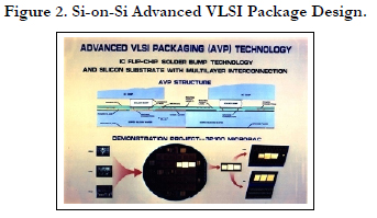
Figure 2. Si-on-Si Advanced VLSI Package Design.
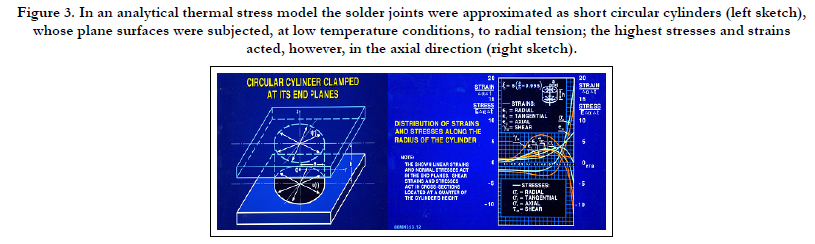
Figure 3. In an analytical thermal stress model the solder joints were approximated as short circular cylinders (left sketch), whose plane surfaces were subjected, at low temperature conditions, to radial tension; the highest stresses and strains acted, however, in the axial direction (right sketch).
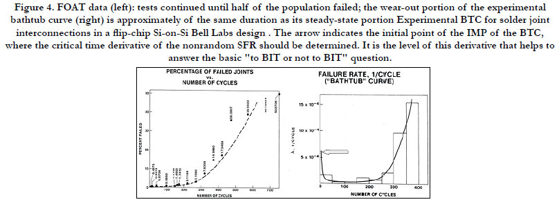
Figure 4. FOAT data (left): tests continued until half of the population failed; the wear-out portion of the experimental bathtub curve (right) is approximately of the same duration as its steady-state portion Experimental BTC for solder joint interconnections in a flip-chip Si-on-Si Bell Labs design . The arrow indicates the initial point of the IMP of the BTC, where the critical time derivative of the nonrandom SFR should be determined. It is the level of this derivative that helps to answer the basic "to BIT or not to BIT" question.
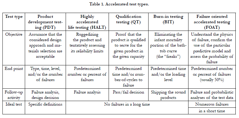

Table 1. Accelerated test types.
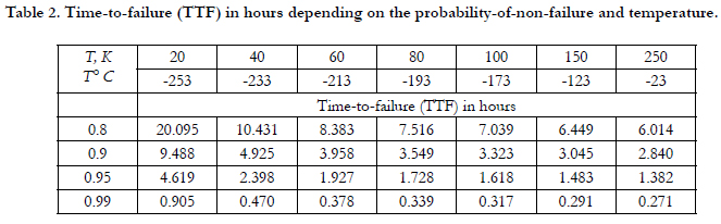
Table 2. Time-to-failure (TTF) in hours depending on the probability-of-non-failure and temperature.
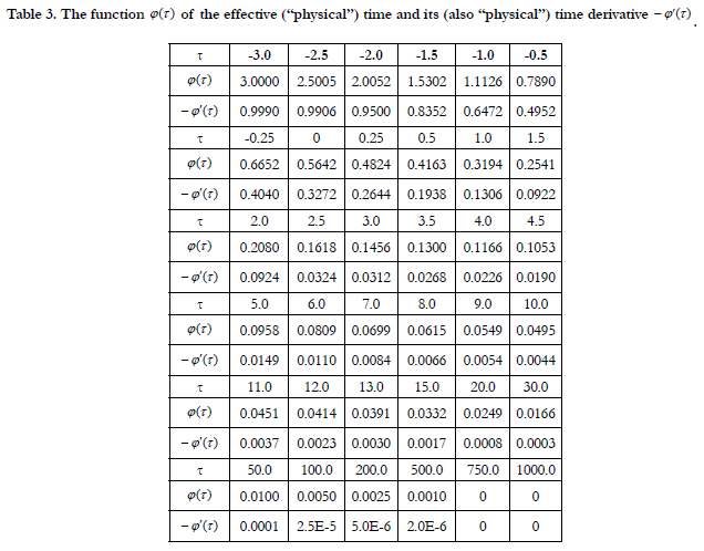
Table 3. The function ϕ (τ ) of the effective (“physical”) time and its (also “physical”) time derivative −ϕ′(τ ) .
Bit Model Based On The Statistical Failure Rate (SFR) Analysis
It is naturally assume that the RFR λ of the numerous mass-produced components that the product of interest is comprised of is normally distributed:
Eq 33
Here λ is the mean value of the RFR λ and D is its variance. Introducing (33) into the formula for the non-random statistical failure rate (SFR) in the BTC and using [100], the expression
Eq 34
for the non-random, “statistical”, SFR, λST(t) can be obtained. The term “statistical” is used here to distinguish, as has been indicated above, this, "favorable", failure rate that decreases with time from the "unfavorable" “physical” failure rate (PFR) that is associated with the material's aging and degradation and increases with time. The PFR is insignificant at the beginning of the IMP of the BTC and is not considered in our analysis. The function
Eq 35
depends on the dimensionless (“physical”, effective) time
Eq 36
and so do the auxiliary function
Eq 37
and the probability integral (Laplace function)
Eq 38
The ratio s in (36) can be interpreted as a sort of a measure of the level of uncertainty of the RFR in question: this value changes from infinity to zero, when the RFR variance D changes from zero (in the case of a deterministic, non-random, failure rate) to infinity (in the case of an "ideally random" failure rate. In the probability theory (see, e.g., [30]) such random process is known as “white noise”.
As evident from the formulas (36), the "physical", effective, time of the RFR process depends not only on the absolute, chronological, "actual", real time t, but also on the mean value λ − and the variance D of the RFR of the mass-produced components that the product of interest is comprised of. We would like to mention in this connection that it is well known, perhaps, from the times of the more than hundred years old Einstein’s relativity theory, that the “physical”, effective, time of an actual physical process or a phenomenon might be different from the chronological, "absolute", time, and is affected by the attributes and the behavior of the particular physical object, process or a system.
The rate of changing of the “physical” time τ with the change in the “chronological” time t is, as follows from the first formula in (36),
Eq 39
Thus, the “physical” time changes faster for larger standard deviations D of the RFR of the mass-produced components that the product of interest is built of.
Considering (39), the formula (34) yields:
Eq 40
As one could see from the first formula in (36), the “physical” time τ is zero, when the “chronological” time t is t D λ = and changes from -∞ to ∞, when the variance D of the RFR of the massproduced components that the product of interest is comprised of changes from zero, i.e., when this failure rate is not random, to infinity, when the RFR is "ideally random", i.e. of a “white noise” type. The calculated values of the function φ(t) expressed by (35) are shown in Table 3. This function changes from to zero when the “physical” time τ changes from to infinity, and the “chronological” time changes from zero to infinity. The tentative derivatives φ'(τ) are also calculated in this table.
The expansion (37) can be used to calculate the auxiliary function Φ(τ ) for large "physical" times τ, exceeding, say, 2.5 and has been indeed employed, when the Table 3 data were computed. The function Φ(τ ) changes from infinity to zero, when the “physical” time τ changes from -∞ to ∞. For the "physical" times τ below -2.5, the function Φ(τ ) is large, and the second term in (35) becomes small compared to the first term. In this case the function φ (τ ) is not different of the “physical” time τ itself, with an opposite sign though. As evident from Table 3, the derivative
can be put, at the initial moment of time, i.e., at the very beginning of the IMP of the BTC equal to -1.0, and therefore the initial time derivative of the SFR is
Eq 41
This fundamental and practically important result explains the physical meaning of the time derivative of the initial failure rate λ1 of the IMP of the BTC: it is the variance (with a sign “minus“, of course) of the RFR of the mass-produced components that the product undergoing BIT is comprised of.
Note that in the simplest case of a uniformly distributed RFR λ, when the probability density distribution function f(λ) is constant, the formula (34) yields:
Eq 42
In such a case the probability of non-failure becomes time independent, i.e. constant over the entire operation range:
This result does not make physical sense, of course, and therefore the normal distribution was accepted in this analysis. Future work should include analyses of the effect of various physically meaningful RFR probability distributions and their effect on the RFR variance. In the analysis carried out in the next section this variance is accepted as a suitable characteristic ("figure of merit") of the propensity of the product under the BIT to the BIT induced failure.
Bit Model Based On Using The Multi-Parametric Baz Equation
The BAZ equation [53-67], geared to the highly focused, highly cost effective, carefully designed, thoroughly conducted and adequately interpreted FOAT, is an important part of the PDfR concept [38-46] recently suggested for M&P products. This concept is intended to be applied at the stage of the development of a new technology for the product of importance. While in commercial E&P reliability engineering it is the cost effectiveness and time-tomarket that are of major importance, in many other areas of engineering, such as aerospace, military, medical, or long-haul communications, highly reliable operational performance of the M&P products is paramount and, because of that, has to be quantified to be improved and assured, and because of various inevitable intervening uncertainties in material properties, environmental conditions, states of stress and strain, etc., such a quantification should be preferably done on the probabilistic basis. Application of the PDfR concept enables predicting from the FOAT data, using BAZ equation, the, in effect, never-zero probability of the field failure of a material, device, package or a system. Then this probability could be made adequate and, if possible and appropriate, even specified for a particular product and application.
The probability of non-failure of a M&P product subjected to BIT, which is, of course, a destructive FOAT for the “freak” population, can be sought, using the BAZ model. Let us show how the appropriate level and duration of the BIT can be determined using the model
Eq 43
Here D is the variance of the RFR of the mass-produced components that the product of interest is comprised of, I is the measured/monitored signal (such as, e.g., leakage current, whose agreed-upon high enough value I* is considered as an indication of failure; or an elevated electrical resistance, particularly suitable when testing solder joint interconnections; or some other suitable physically meaningful and measurable quantity), t is time, σ is the appropriate “external” stressor, U0 is the stress-free activation energy, T is the absolute temperature, γσ is the stress sensitivity factor and γt is the time/variance sensitivity factor.
There are three unknowns in the expression (30): the product ; tρ =γ D the stress-sensitivity factor γσ and the activation energy U0. These unknowns could be determined from a two-step FOAT. At the first step testing should be carried out for two temperatures, T1 and T2, but for the same effective activation energy 0 U U σ = −γ σ . Then the relationships
Eq 44
for the probabilities of non-failure can be obtained. Here t1,2 are the corresponding times and I* is, say, the leakage current at the moment and as indication of failure. Since the numerator U = U0 - γσ in the relationships (44) is kept the same, the product ρ = γt - D can be found as
Eq 45 and 46
are used. The second step of testing should be conducted at two stress levels σ1 and σ2 (say, temperatures or voltages). If these stresses are thermal stresses that are determined for the temperatures T1 and T2, they could be evaluated using a suitable thermal stress model. Then
Eq 47
If, however, the external stress is not a thermal stress, then the temperatures at the second step tests should preferably be kept the same. Then the ρ value will not affect the factor γσ, which could be found as
Eq 48
where T is the testing temperature. Finally, the activation energy U0 can be determined as
Eq 49
The time to failure (TTF) is probability-of-failure dependent and can be determined as
TTF = MTTF(−ln P), where the MTTF is
Eq 50
Let, e.g., the following data were obtained at the first step of FOAT: 1) After t1 = 14h of testing at the temperature of T1 = 60°C = 333° K, 90% of the tested devices reached the critical level of the leakage current of I* = 3.5μA and, hence, failed, so that the recorded probability of non-failure is P1 = 0.1; the applied stress is elevated voltage σ1 = 380V; and 2) after t2 = 28h of testing at the temperature of T2 = 85° C = 358° K, 95% of the samples failed, so that the recorded probability of non-failure is P2 = 0.05. The applied external stress is still elevated voltage of the level σ1 = 380V. Then the formulas (33) yield:
Eq P
can be found from the formula (45) as follows:
Eq Q
At the FOAT's second step one can use, without conducting additional testing, the above information from the first step, its duration and outcome, and let the second step of testing has shown that after t2 = 36h of testing at the same temperature of T = 60°C = 333° K, 98% of the tested samples failed, so that the predicted probability of non-failure is P2 = 0.02. If the stress σ2 is the elevated voltage σ2 = 220V, then
Eq R
To make sure that there is no calculation error, the activation energies could be evaluated, for the calculated parameters n1 and n2 and the stresses σ1 and σ2, in two ways:
Eq S
No wonder that these values are considerably lower than the activation energies for the “healthy” products. As is known, many manufacturers consider as a sort of a “rule of thumb” that the level of 0.7eV can be used as an appropriate tentative number for the activation energy of “healthy” electronic products. In this connection it should be indicated that when the BIT process is monitored and the supposedly stress free activation energy U0 is being continuously calculated based on the number of the failed devices, the BIT process should be terminated, when the calculations, based on the FOAT data, indicate that the energy U0 starts to increase: this is an indication that the “freaks”, which are characterized by low activation energies, have been eliminated, and BIT is “invading” the domain of the “healthy” products. Note that the calculated data show also that the activation energy is slightly higher, by about 5-8%, for a higher level of stressing, i.e., is not completely loading independent. We are going to explain and account for this phenomenon as part of the future work.
The MTTF can be determined using the formula (37):
Eq T
The calculated probability-of-non-failure dependent time-tofailurte (lifetime) TTF =MTTFx (ln P) is 79.2h for P = 0.0075, is 74.5h for P = 0.0100 and is 48.5h for P = 0.050. Clearly, the probabilities of non-failure for a successful BIT, which is, actually, a carefully designed and effectively conducted FOAT, should be low enough. It is clear also that the BIT process should be terminated when the (continuously calculated during testing) probabilities of non-failure start rapidly increasing. How rapidly is “rapidly” should be specifide for a particular product, manufacturing technology and the accepted BIT process.
Conclusions
The following conclusions could be drawn from the above analysis.
• Predictive modeling should always precede the actual FOAT of
any type to make such testing physically meaningful, effective and
low cost.
• The bathtub-curve (BTC) based time-derivative of the statistical
failure rate (SFR) at the initial moment of time can be considered
as a suitable criterion ("figure-of-merit") of whether BIT for a
packaged IC device should or does not have to be conducted.
This derivative is, actually, the variance of the random failure rate
(RFR) of the mass-produced components that the manufacturer
of the product of interest received from various and numerous
vendors, whose commitments to reliability were unknown, and
therefore the RFR of these components might very well vary significantly,
from zero to infinity. This information enables answering
the fundamental “to BIT or not to BIT” question in electronics
manufacturing.
• Our analysis sheds light on the role and significance of several
important factors that affect the testing time and stress level: the
RFR of mass-produced components that the product of interest
is comprised of; the way to assess, from the highly focused and
highly cost effective failure-oriented-accelerated testing (FOAT),
the activation energy of the “freak” BIT population; the role of
the applied stressor(s); and, most importantly, - the probabilities
of the “freak” population failures depending on the duration and
level of the BIT effort. These factors should be considered when there is an intent to quantify and, eventually, to optimize the BIT’s
procedure.
• BAZ-based approach that was employed for that could be used
in many practically important undertakings and tasks, even beyond
the electronics engineering field, when quantification of a
materials reliability related problem is needed, and uncertain operation
conditions are inevitable and should be accounted for.
• The calculated data show also that the activation energy is slightly
higher, by about 5-8%, for a higher level of stressing, i.e., not
completely loading independent. We are going to explain and account
for this phenomenon as part of the future work as well.
• FOAT, being a transparent and reliability-physics-based “white/
transparent box”, can be viewed as an extension and a modification
of the forty-years-old and still highly (and justifiably) popular
highly-accelerated-life-testing (HALT). This “black box” has
many merits, but does not quantify reliability. In many cases, and
particularly, for new products, FOAT can and should be run even
as a substitution of HALT, especially for new products, for which
no experience is yet accumulated and best practices are not developed.
• Future work should include experimental verifications of the
suggested “to BIT or not to BIT” criterion, as well as its acceptable
values. It should include also investigation of the effects of
other possible distributions of the random SFR, such as, e.g., Rayleigh
or Weibull, and understanding that, in reality, there is no
such thing as loading independent activation energy: it looks like
this energy is slightly higher for higher loadings.
References
-
[1]. Van Rossum M. The Future of Microelectronics: Evolution or Revolution?.
Microelectron Eng. 1996 Dec 1;34(1):125-34.
[2]. Chatterjee PK, Doering RR. The future of microelectronics. Proceedings of the IEEE. 1998 Jan;86(1):176-83.
[3]. Suhir E. The Future of Microelectronics and Photonics and the Role of Mechanics and Materials. ASME J Electr Packaging (JEP). 1998.
[4]. Ziemelis K. The Future of Microelectronics. Nature. 2000 Aug 31;406(6799):1021.
[5]. Suhir E. Microelectronics and Photonics - the Future. In 2000 22nd International Conference on Microelectronics. Proceedings (Cat. No. 00TH8400). 2000 May 14;1:3-17.
[6]. Suhir E. Accelerated life testing (ALT) in microelectronics and photonics: its role, attributes, challenges, pitfalls, and interaction with qualification tests. J Electron Packag. 2002 Sep 1;124(3):281-91.
[7]. Duane JT, Collins DH, Jason K, Freels JK, Huzurbazar AV, Warr RL, et al. Accelerated Test Methods for Reliability Prediction. IEEE Trans Aerospace. 1964.
[8]. Nelson WB. Accelerated testing: statistical models, test plans, and data analysis. John Wiley & Sons; 2009 Sep 25.
[9]. Matisoff B. Handbook of Electronics Manufacturing Engineering. Springer Science & Business Media; 2012 Dec 6.
[10]. Ebeling CE. An introduction to reliability and maintainability engineering. Waveland Press; 2019 Apr 12.
[11]. Katz A, Pecht M, Suhir E. Accelerated testing in microelectronics: review, pitfalls and new developments. InProceedings of the International Symposium on Microelectronics and Packaging, IMAPS, Israel 2000 Jun.
[12]. Suhir E. Reliability and Accelerated Life Testing. Semiconductor International; 2005.
[13]. Suhir E, Mahajan R. QA MODELING-Are Current Qualification Practices Adequate?. Circuits Assembly. 2011;28(4):26.
[14]. Suhir E, Yi S. Accelerated Testing and Predicted Useful Lifetime of Medical Electronics. InHandlery Hotel, San-Diego, IMAPS Conf. on Advanced Packaging for Medical Electronics 2017.
[15]. Suhir E. Making a Viable Electron Device into a Reliable Product: Brief Review. Brief Note, J Electron Commun. 2020;(5).
[16]. Kececioglu D, Sun FB. Burn-in testing: its quantification and optimization. Prentice Hall; 1997.
[17]. Vollertsen RP. Burn-in. In1999 IEEE International Integrated Reliability Workshop Final Report (Cat. No. 99TH8460).1999.
[18]. Burn-In MI. 883F: Test Method Standard, Microchips, Method 1015.9, US Dept.
[19]. Noel M, Dobbin A, Van Overloop D. Reducing the Cost of Test in Burnin- An Integrated Approach. InProceedings of the Burn-in and Test, Socket Workshop, Mesa, AZ, USA 2004.
[20]. Ooi MP, Kassim ZA, Demidenko SN. Shortening burn-in test: Application of HVST and Weibull statistical analysis. IEEE Transactions on instrumentation and measurement. 2007 May 15;56(3):990-9.
[21]. Ng YH, Low YH, Demidenko S. Improving efficiency of IC burn-In testing. In2008 IEEE Instrumentation and Measurement Technology Conference. 2008 May 12;1685-1689.
[22]. Suhir E. To Burn-in, or not to Burn-in: That’s the Question. Aerospace. 2019 Mar 6;6(3):29.
[23]. Suhir E. Burn-in Testing (BIT): Is It Always Needed?. IEEE ECTC, Orlando, Fl. 2020.
[24]. Suhir E. Mechanical behavior and reliability of solder joint interconnections in thermally matched assemblies. In1992 Proceedings 42nd Electronic Components & Technology Conference. 1992 May 18; 563-572.
[25]. Suhir E. Failure-oriented-accelerated-testing (FOAT) and its role in making a viable IC package into a reliable product. Circuits Assembly, July. 2013 Jul.
[26]. Suhir E. Could electronics reliability be predicted, quantified and assured?. Microelectronics Reliability. 2013 Jul 1;53(7):925-36.
[27]. Suhir E, Bensoussan A, Nicolics J, Bechou L. Highly accelerated life testing (HALT), failure oriented accelerated testing (FOAT), and their role in making a viable device into a reliable product. In2014 IEEE Aerospace Conference, Big Sky, Montana 2014 Mar.
[28]. Suhir E. Failure-Oriented-Accelerated-Testing (FOAT), Boltzmann-Arrhenius- Zhurkov Equation (BAZ) and Their Application in Microelectronics and Photonics Reliability Engineering. Int J Aeronautical Sci Aerospace Res (IJASAR). 2019;6(3).
[29]. Suhir E, Ghaffarian R. Electron device subjected to temperature cycling: predicted time-to-failure. J Electron Mater. 2019 Feb;48(2):778-9.
[30]. Suhir E. Applied Probability for Engineers and Scientists. McGraw-Hill: New York; 1997.
[31]. Suhir E. Probabilistic design for reliability. Chip Scale Reviews. 2010 Nov;14(6):24-8.
[32]. Suhir E. Remaining useful lifetime (rul): Probabilistic predictive model. Int J Progn Health Monit (PHM). 2011;2:140.
[33]. Suhir E, Mahajan R, Lucero A, Bechou L. Probabilistic Design for Reliability (PDfR) and a Novel Approach to Qualification Testing (QT)‖, 2012 IEEE/AIAA Aerospace Conf., Big Sky. Montana. 2012.
[34]. Suhir E. Assuring electronics reliability: What could and should be done differently. In2013 IEEE Aerospace Conference 2013. IEEE.
[35]. Suhir E. Considering electronic product’s quality specifications by application (s). Chip Scale Reviews. 2012 Jul;16(4).
[36]. Suhir E. Probabilistic Design for Reliability of Electronic Materials, Assemblies, Packages and Systems: Attributes, Challenges, Pitfalls. InMMCTSE 2017 Feb 24.
[37]. Suhir E, Ghaffarian R, Yi S. Solder material experiencing low temperature inelastic stress and random vibration loading: predicted remaining useful lifetime. Journal of Materials Science: Materials in Electronics. 2017 Feb;28(4):3585-97.
[38]. Suhir E. Probabilistic Design for Reliability (PDfR) of Aerospace Instrumentation: Role, Significance, Attributes, Challenges, 5th IEEE Int. In- Workshop on Metrology for Aerospace (MetroAeroSpace), Rome, Italy, Plenary Lecture 2018.
[39]. Suhir E. Physics of Failure of an Electronics Product Must Be Quantified to Assure the Product's Reliability. Acta Scientific Applied Physics. 2021;2(1).
[40]. Suhir E. Remaining useful lifetime (rul): Probabilistic predictive model. Int J Progn Health Monit (PHM). 2011;2:140.
[41]. Suhir E. Could electronics reliability be predicted, quantified and assured?. Microelectronics Reliability. 2013 Jul 1;53(7):925-36.
[42]. Suhir E. Predictive modeling is a powerful means to prevent thermal stress failures in electronics and photonics. Chip Scale Reviews. 2011 Jul;15(4).
[43]. Suhir E. Electronic Product Qual Specs Should Consider Its Most Likely Application (s). Chip Scale Reviews. 2012 Jul;16:01-8.
[44]. Suhir E. When reliability is imperative, ability to quantify it is a must. IMAPS Advanced Microelectronics. 2013.
[45]. Suhir E. Predicted reliability of aerospace electronics: Application of two advanced probabilistic concepts. In2013 IEEE Aerospace Conference 2013.
[46]. Suhir E. Statistics-related and reliability-physics-related failure processes in electronics devices and products. Modern Physics Letters B. 2014 May 30;28(13):1450105.
[47]. Suhir E. Analytical bathtub curve with application to electron device reliability. Journal of Materials Science: Materials in Electronics. 2015 Sep;26(9):6633-8.
[48]. Suhir E, Bensoussan A. Degradation related failure rate determined from the experimental bathtub curve. InProceedings of the SAE Conference, Seattle, WA, USA 2015.
[49]. M. Silverman, "Forty Years of HALT: What Have We Learned?" IEEE EPS ASTR 2012 Oct 17-19, Toronto, CA 2012.
[50]. "Fundamentals of HALT/HASS Testing" (PDF). Keithley Instruments, Inc. Cleveland, Ohio. 2000.
[51]. "What is HALT HASS: Performing HALT". Qualmark Corporation. Archived from the original on March 1, 2012. Retrieved 10 June 2012.
[52]. N. Doertenbach. "The Application of Accelerated Testing Methods and Theory (HALT and HASS)". Qual Mark Corporation. Archived from the original on 2012.
[53]. Boltzmann L. On the Mechanical Significance of the Second Law of the Theory of Heat: (presented at the session of February 8, 1866). State Printing Office; 1866.
[54]. Boltzmann L. Studies on the balance of the living force. Wissenschafiliche Abhandlungen. 1868;1:49-96.
[55]. Boltzmann L. The Second Law of Thermodynamics. Populare Schriften, Essay 3, Address to a Formal Meeting of the Imperial Academy of Science, 29 May 1886.
[56]. Arrhenius S. Research on the galvanic conductivity of electrolytes. PA Norstedt & Söner; 1884.
[57]. Arrhenius S. Über die Dissociationswärme und den Einfluss der Temperatur auf den Dissociationsgrad der Elektrolyte. Z Phys Chem. 1889 Jul 1;4(1):96-116.
[58]. S. N. Zhurkov, (The Problem of the Strength of Solids), Vestnik Akad. Nauk SSSR (Bulletin of the USSR Academy of Sciences), 11, 1957 (in Russian). [59]. Zhurkov SN. Kinetic concept of the strength of solids. Int J Fracture Mech. 1965 Dec;1(4):311-23.
[60]. Suhir E, Kang SM. Boltzmann–Arrhenius–Zhurkov (BAZ) model in physics-of-materials problems. Modern Physics Letters B. 2013 May 30;27(13):1330009.
[61]. Suhir E, Bechou L, Bensoussan A. Technical Diagnostics in Electronics: Application of Bayes Formula and Boltzmann-Arrhenius-Zhurkov (BAZ) Model. Printed Circuit Design& Fab/Circuits Assembly. 2012 Dec;29(12):25-8.
[62]. Suhir E, Bensoussan A. Application of multi-parametric BAZ model in aerospace optoelectronics. In2014 IEEE Aerospace Conference, Big Sky, Montana 2014 Mar.
[63]. Suhir E. Three-step concept in modeling reliability: Boltzmann–Arrhenius– Zhurkov physics-of-failure-based equation sandwiched between two statistical models. Microelectron. Reliab. 2014 Oct;54:2594-603.
[64]. Suhir E. Static fatigue lifetime of optical fibers assessed using Boltzmann– Arrhenius–Zhurkov (BAZ) model. Journal of Materials Science: Materials in Electronics. 2017 Aug;28(16):11689-94.
[65]. Ponomarev A, Suhir E. Predicted useful lifetime of aerospace electronics experiencing ionizing radiation: Application of BAZ model. Journal of Aerospace Engineering and Mechanics (JAEM). 2019;3(1).
[66]. Suhir E. Boltzmann-Arrhenius-Zhurkov Equation and Its Applications In Electronic-and-Photonic Aerospace Materials Reliability-Physics Problems. IJASAR. 2020.
[67]. Suhir E, Stamenkovic Z. Using yield to predict long-term reliability of integrated circuits: Application of Boltzmann-Arrhenius-Zhurkov model. Solid- State Electronics. 2020 Feb 1;164:107746.
[68]. Suhir E. Analytical Modeling in Electronic Packaging Structures: Its Merits, Shortcomings and Interaction with Experimental and Numerical Techniques. ASME Journal of Electronic Packaging. 1989.
[69]. Suhir E. Modeling of thermal stress in microelectronic and photonic structures: Role, attributes, challenges, and brief review. J Electron Packag. 2003 Jun 1;125(2):261-7.
[70]. Suhir E. Analytical Thermal Stress Modeling in Electronic and Photonic Systems", ASME Applied Mechanics Reviews, 62(4), 2009.
[71]. Suhir E. Thermal stress failures: Predictive modeling explains the reliability physics behind them. Advancing Microelectronics. 2011;38(4):12-22.
[72]. Suhir E. Could electronics reliability be predicted, quantified and assured?. Microelectronics Reliability. 2013 Jul 1;53(7):925-36.
[73]. E. Suhir, “Analytical Modeling Enables Explanation of Paradoxical Situations in the Behavior and Performance of Electronic Materials and Products: Review”, Journal of Physical Mathematics 7(1), Dec. 2015.
[74]. Suhir E. Analytical modeling occupies a special place in the modeling effort. Journal of Physical Mathematics. 2016 Jan;7(1):1-2.
[75]. Hall P. Forces, moments, and displacements during thermal chamber cycling of leadless ceramic chip carriers soldered to printed boards. IEEE Transactions on Components, Hybrids, and Manufacturing Technology. 1984 Dec;7(4):314-27.
[76]. Suhir E. Mechanical reliability of flip-chip interconnections in silicon-onsilicon multichip modules. InIEEE Conference on Multichip Modules. 1993.
[77]. Suhir E. Analysis of a pre‐stressed bi‐material accelerated‐life‐test (ALT) specimen. ZAMM‐Journal of Applied Mathematics and Mechanics. 2011 May 3;91(5):371-85.
[78]. Suhir E. Low-Cycle-Fatigue Failures of Solder Material in Electronics: Analytical Modeling Enables to Predict and Possibly Prevent Them-Review. J Aerosp Eng Mech. 2018;2(1).
[79]. Gopalakrishna H, Sinha A, Jordan D, Tamizhmani G. Activation energy for solder bond degradation: Thermal cycling of field-aged modules at multiple upper temperatures. In2019 IEEE 46th Photovoltaic Specialists Conference (PVSC) 2019. IEEE.
[80]. Suhir E, Ghaffarian R. Electron device subjected to temperature cycling: predicted time-to-failure. Journal of Electronic Materials. 2019 Feb;48(2):778-9.
[81]. Suhir E. Twist-off Testing of Solder Joint Interconnections. ASME J Electr Packaging (JEP). 1989;111(3).
[82]. Zhang Y, Suhir E, Xu Y, Gu C. Bonding strength of a carbon nanofiber array to its substrate. JMR. 2006 Nov;21(11):2922-6.
[83]. Suhir E. Bonded Tri-Material Specimen Subject-ed to Shear-Off Testing: Predicted Interfacial Stresses. J Aerosp Eng Mech. 2020;4(1):201-5.
[84]. Suhir E. Bi-material assembly subjected to thermal stress: propensity to delamination assessed using interfacial compliance model. Journal of Materials Science: Materials in Electronics. 2016 Jul;27(7):6779-85.
[85]. Suhir E, Morris JE, Wang L, Yi S. Could dynamic strength of a bonding material in an electronic device be assessed from static shear-off test data?. Journal of Materials Science: Materials in Electronics. 2016 Jul;27(7):6697-702.
[86]. Suhir E. Is the maximum acceleration an adequate criterion of the dynamic strength of a structural element in an electronic product?. IEEE Transactions on Components, Packaging, and Manufacturing Technology: Part A. 1997 Dec;20(4):513-7.
[87]. Zhou CY, Yu TX, Suhir E. Design of shock table tests to mimic real-life drop conditions. IEEE Transactions on Components and Packaging Technologies. 2009 Oct 30;32(4):832-7.
[88]. Suhir E, Shakouri A. Assembly bonded at the ends: Could thinner and longer legs result in a lower thermal stress in a thermoelectric module design?. ASME J Appl Mech. 2012 Nov 1;79(6).
[89]. Suhir E, Shangguan D, Bechou L. Predicted thermal stresses in a trimaterial assembly with application to silicon-based photovoltaic module. J Appl Mech. 2013 Mar 1;80(2).
[90]. Suhir E, Bechou L, Levrier B. Predicted size of an inelastic zone in a ballgrid- array assembly. J Appl Mech. 2013 Mar 1;80(2).
[91]. Suhir E. Analysis of a short beam with application to solder joints: could larger stand-off heights relieve stress?. The European Physical Journal Applied Physics. 2015 Aug 1;71(3):31301.
[92]. Suhir E, Ghaffarian R, Nicolics J. Could application of column-grid-array (CGA) technology result in inelastic-strain-free state-of-stress in solder material?. Journal of Materials Science: Materials in Electronics. 2015 Dec;26(12):10062-7.
[93]. Suhir E, Ghaffarian R. Column-grid-array (CGA) versus ball-grid-array (BGA): board-level drop test and the expected dynamic stress in the solder material. Journal of Materials Science: Materials in Electronics. 2016 Nov;27(11):11572-82.
[94]. Suhir E, Bechou L. Availability index and minimized reliability cost. Circuit Assemblies. 2013 Feb.
[95]. Suhir E. Axisymmetric Elastic Deformations of a Finite Circular Cylinder with Application to Low Temperature Strains and Stresses in Solder Joints. ASME J of Appl Mech. 1989;56(2).
[96]. Suhir E, Ghaffarian R, Yi S. Solder material experiencing low temperature inelastic stress and random vibration loading: predicted remaining useful lifetime. Journal of Materials Science: Materials in Electronics. 2017 Feb;28(4):3585-97.
[97]. Suhir E, Poborets B. Solder-glass attachment in cerdip/cerquad packages: Thermally induced stresses and mechanical reliability. In 40th Conference Proceedings on Electronic Components and Technology, 1990.
[98]. Suhir E, Tunik A. Russian Strength Standards for Commercial Ships. American Bureau of Shipping; 1982.
[99]. E.Suhir, “Probabilistic Methods in Structural Analysis and Vibration of Ships”. Institute of Naval Architecture, Nikolayev, Ukraine 1974 (in Russian). [100]. Gradshteyn IS, Ryzhik IM, Romer RH. Tables of integrals, series, and products. Academic Press; 1980.