Boltzmann-Arrhenius-Zhurkov Equation and Its Application in Aerospace Electronicsand-Photonics Reliability Physics Problems: Review
E. Suhir*
Portland State University, Department of Mechanical and Mathematics, and Electronics and Computers Engineering, Portland, OR, USA.
Technical University, Department of Applied Electronic Materials, Institution of Sensors and Actuators, Vienna, Austria.
*Corresponding Author
E. Suhir,
Portland State University, Department of Mechanical and Mathematics, and Electronics and Computers Engineering, Portland, OR, USA.
Technical University, Department of Applied Electronic Materials, Inst. of Sensors and Actuators, Vienna, Austria.
Tel: Tel: 6509691530/408-410-0886
Email: suhire@aol.com
Received: February 18, 2020; Accepted: March 11, 2020; Published: March 24, 2020
Citation:E. Suhir. Boltzmann-Arrhenius-Zhurkov Equation and Its Application in Aerospace Electronics-and-Photonics Reliability Physics Problems: Review. Int J Aeronautics Aerospace Res. 2020;7(1):210-223. doi: dx.doi.org/10.19070/2470-4415-2000026
Copyright: E. Suhir© 2020. This is an open-access article distributed under the terms of the Creative Commons Attribution License, which permits unrestricted use, distribution and reproduction in any medium, provided the original author and source are credited.
Abstract
Application of Boltzmann-Arrhenius-Zhurkov (BAZ) equation in electronics-and-photonics (EP) reliability-physics (RP) problems enables quantifying, on the probabilistic basis, the performance (actually, the never-zero probability of failure under the anticipated loading conditions and after the given time in operation) of an EP material, thereby making a viable device into a reliable product, with the predicted, adequate and, when necessary and appropriate, even specified probability of failure in the field. The following EP RP problems are addressed with an objective to show the significance and attributes of the approach based on the BAZ equation: 1) an EP package subjected to the combined action of two or more stressors (such as, say, elevated humidity and voltage); 2) three-step concept (TSC) in modeling reliability, when the RP-based BAZ equation is sandwiched between two well-known statistical models - Bayes formula (BF) and beta-distribution (BD); 3) static fatigue of an optical silica fiber intended for high-temperature applications; 4) low-cycle fatigue life-time of solder joint interconnections; 5) life-time of electron devices predicted from the yield information and 6) some important aspects of burn-in testing (BIT) of manufactured EP products comprised of many mass-produced components. The general concepts and analyses are illustrated by practical numerical examples.
2.Introduction: Multi-parametric BAZ Equation
3.Review
4.Predicted Static Fatigue Lifetime of an Optical Silica Fiber
5.Predicted Low-Cycle Fatigue Life-Time Of Solder Joint Interconnections
6.Predicted Long-Term Reliability of IC Devices From Yield Information
7.Use of BAZ equation to quantify BIT effort
8.Conclusion
9.References
Acronyms
BAZ = Boltzmann-Arrhenius-Zhurkov (equation); BD = Beta Distribution; BIT = Burn-in Testing; BTC = Bathtub Curve; EP = Electronics and photonics; FOAT = Failure Oriented Accelerated Testing; HALT = Highly Accelerated Life Testing; IMP = Infant Mortality Portion (of the BTC); MTTF = Mean Time To Failure; PDfR = Probabilistic Design for Reliability; RP = Reliability Physics; RUL = Remaining Useful Life; SFR = Statistical Failure Rate; TSC = Three- Step-Concept; TTF = Time to Failure.
Introduction: Multi-parametric BAZ Equation
Boltzmann-Arrenius-Zhurkov (BAZ) equation [1, 2]
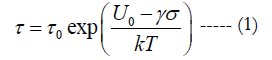
has been suggested by the Russian physisist S.N. Zhurkov in 1957 in application to experimental fracture mechanics problems as the generalization of the Arrhenius equation [3].
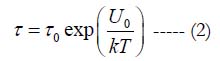
by the Swedish chemist S. Arrhenius in 1889 in the kinetic theory of chemical reactions (1903 Nobel Prize in chemistry). The equations (1) and (2) consider the role of the ratio U0/kT of the activation energy U0 (the term was coined by Arrhenius to characterize materials’ propensity to get engaged into a chemical reaction),to the thermal energy kT evaluated as the product of the Boltzmann’s constant k = 8.6173303x 10⁻⁵ eV/K and the absolute temperature T. In the above equations, τ is the mean time to failure (MTTF), τ0 is the time constant, and σ is the applied stress per unit volume. The equation (2) is formally not different of what is known as Boltzmann’s or Maxwell-Boltzmann’s statistics [4, 5] in the kinetic theory of gases. This theory postulates that the absolute temperature of an ideal gas, when it is in thermodynamic equilibrium with the environment, is determined by the average probability of the collisions of the gas particles (atoms or molecules) and that the higher this probability is, the higher is the gas temperature. Chemist Arrhenius was member of physicist Boltzmann’s team in the University of Graz, Austria, in 1887 and suggested that Boltzmann’s equation (2) be used to assess the height of the energy barrier, the activation energy, which had to be got over to trigger a chemical reaction. The effective activation energy.
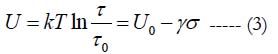
plays in the BAZ equation (1) the same role as the stress-free energy U0 plays in the Arrhenius equation (2). It has been recently shown [6] that the equations (1) and (2) can be obtained as steadystate solutions to the Fokker-Planck equation in the theory of Markovian processes (see, e.g., [7]), and that these solutions represent the worst case scenarios, so that the reliability predictions based on the steady-state BAZ model (1) are reasonably conservative and, hence, advisable for engineering applications.
Zhurkov and his associates used the equation (1) to determine the fracture toughness of a large number of materials experiencing combined action of elevated temperature (affecting long-term material’s degradation) and external mechanical loading (affecting the short term strength of the material). In Zhurkov’s tests the loading σ was always a constant mechanical tensile stress, and the test specimens were always notched ones. It has been recently suggested that any other loading (stressor, stimulus) of importance (voltage, current, thermal stress, humidity, vibrations, radiation, light output, etc.) can also be used as an appropriate stressor, when short term reliability of EP products is evaluated, and that, since the principle of superposition does not work in RP, even a combination of relevant stimuli can be considered [8]. This suggestion has been done in connection with the development of a concept of the probabilistic design for reliability (PDfR) [9-13] of EP materials, devices, assemblies, packages and systems.
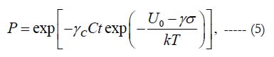
The PDfR concept quantifies, on the probabilistic basis and using BAZ model, the lifetime of an EP product from highly focused and highly cost-effective failure-oriented-accelerated-testing (FOAT) [14-16]. The τ value is viewed in the BAZ model (1) as the mean-time-to-failure (MTTF). This suggests that when the exponential law.
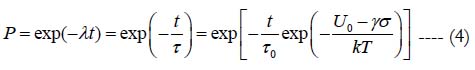
of the probability of non-failure is used, the MTTF τ corresponds to the moment of time when the entropy H(P) of the distribution (4) reaches its maximum value. Indeed, from H(P) = -Pln P it could be obtained that the function H(P) reaches its maximum value Hmax = e-1 for P = e-1 = 0.3679. In such a situation the equation (4) yields: t = τ0 exp (U/kT). Comparing this result with the equation (1) we conclude that the MTTF expressed by this equation corresponds to the moment of time when the entropy H(P) of the process P = P(t) is the largest and is also equal to e-1.
When a suitable FOAT is considered, designed and conducted, the time constant τ0 in the double-exponential distribution (4) could be replaced, in reliability evaluations, by a quantity (γcCt)-1, where t is time, C is a suitable criterion of failure (such as, say, elevated leakage current or high electrical resistance) and γc is the sensitivity factor. Then the distribution (4) can be replaced by the expression.
or, in the case of multiple loadings, by the expression
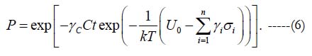
This multi-parametric BAZ equation has been recently employed in application to several critical EP RP problems. Some of them are addressed in this review, namely, 1) an EP subjected to the combined action of two or more stressors (such as, say, elevated humidity and voltage) [17]; 2) three-step concept (TSC) in modeling reliability, when RP related BAZ equation is sandwiched between two statistical models (Bayes formula and beta-distribution (BD)) [18, 19]; 3) FOAT static fatigue of optical silica fibers [20, 21]; 4) predicted low-cycle fatigue life-time of solder joint interconnections [22, 23]; 5) predicted long-term reliability of IC devices using yield information [24, 25] and 6) some important aspects of the BIT technologies [26-28] in electronics manufacturing, with an emphasis is on the possible roles that the FOAT, geared to the BAZ equation, could play in predicting the appropriate time and level of the BIT effort, if such testing is found to be necessary [29].
All the solutions in these analyses were obtained using analytical (”mathematical”) modeling [30-33]. In the author’s opinion, such modeling should always be considered and should complement computer simulations: if the results obtained using these two approaches (which are, as a rule, based on different assumptions and use different techniques), are in agreement, then there is a good reason to believe that the obtained results are both accurate and trustworthy.
Let us consider the action of two stressors: elevated humidity H and elevated voltage V. If the level I* of the leakage current is accepted as the suitable criterion of failure, the equation (6) can be written as:
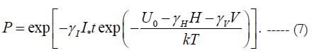
This equation contains four empirical parameters: the stress-free activation energy U0 and three sensitivity factors γ, the leakage current factor γ1, the relative humidity factor γH and the elevated voltage factor γV. At the first step one should conduct the FOAT for two temperatures, T1 and T2 while keeping the levels of the relative humidity H and the elevated voltage V the same. Assuming a certain level I* of the monitored/measured leakage current as the criterion of failure and recording the percentages P1 and P2 of non-failed samples, the equation (7) yields:
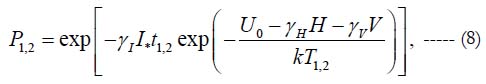
where t1 and t2 are the testing times and T1 and T2 are the temperatures, at which the failures were observed. Since the numerators in these relationships are the same, the equation:
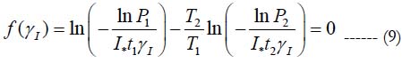
must be fulfilled and used to determine the sensitivity factor γ1. At the second step, testing at two relative humidity levels H1 and H2 should be conducted for the same temperature and voltage. This enables to determine the sensitivity factor γH. Similarly, the sensitivity factor γv can be then determined for two voltage levels V1 and V2. The stress-free activation energy U0 can be then determined from (7) for any consistent humidity, voltage, temperature and time as .jpg)
If, e.g., after t1 = 35h of testing at the temperature T1 = 60°C = 333° K, the voltage V = 600V and the relative humidity of H = 0.85, 10% of specimens reached the critical level I* = 3.5μA of the leakage current and, hence, failed, then P1 = 0.9; and if after t2 = 70h of testing at the temperature T2 = 85° C = 358K at the same relative humidity and voltage, 20% of the tested samples failed, so that P2 = 0.8, then the equation (10) becomes .jpg) Its solution is
Its solution is .jpg) so that
so that .jpg) Tests at the second step are conducted for two relative humidity levels H1 and H2, while keeping the temperature and voltage the same. This results in the formula
Tests at the second step are conducted for two relative humidity levels H1 and H2, while keeping the temperature and voltage the same. This results in the formula .jpg) . If 5% of the specimens fail after t1 = 40h If 5% of the specimens fail after H1 = 0.5, the voltage V = 600V and temperature T = 60°C = 333K (P1=0.95), and 10% of the specimens failed (P2 = 0.9), afte t2 = 55h of testing at the same temperature, but at the relative humidity of H2 = 0.85, then the above formula yields: γH = 0.03292eV. At the third step, testing at two voltage levels V1 = 600V and V2 = 1000V is carried out for the same temperaturehumidity bias at T = 85°C = 358K and H = 0.85, and 10% of the specimens failed after t1 = 40h of testing (P1 = 0.9) and 20% of the specimens failed after t2 = 80h of testing (P2 = 0.8), then the sensitivity facto γV for voltage can be obtained from the expression and the stress-free activation energy can be determined as follows:
. If 5% of the specimens fail after t1 = 40h If 5% of the specimens fail after H1 = 0.5, the voltage V = 600V and temperature T = 60°C = 333K (P1=0.95), and 10% of the specimens failed (P2 = 0.9), afte t2 = 55h of testing at the same temperature, but at the relative humidity of H2 = 0.85, then the above formula yields: γH = 0.03292eV. At the third step, testing at two voltage levels V1 = 600V and V2 = 1000V is carried out for the same temperaturehumidity bias at T = 85°C = 358K and H = 0.85, and 10% of the specimens failed after t1 = 40h of testing (P1 = 0.9) and 20% of the specimens failed after t2 = 80h of testing (P2 = 0.8), then the sensitivity facto γV for voltage can be obtained from the expression and the stress-free activation energy can be determined as follows:
.jpg)
No wonder that the third term in this equation plays the dominant role, so that, in approximate analysis, only this term could be considered. Calculations indicate that the loading free activation energy U0 in the above numerical example (even with the rather tentative, but still realistic, input data) is about U0 = 0.5eV. This result is consistent with the existing experimental data. Indeed, for semiconductor device failure mechanisms the activation energy ranges from 0.3eV to 0.6eV, for metallization defects and electro-migration in Al it is about 0.5eV, for charge loss it is on the order of 0.6eV, for Silicon junction defects it is 0.8eV. The following expression for the probability of non-failure .jpg) can be obtained in this example from the distribution (8). If, e.g., t = 10h,
H = 0.20, V = 220, and the operation temperature is T = 70°C = 343K, then
can be obtained in this example from the distribution (8). If, e.g., t = 10h,
H = 0.20, V = 220, and the operation temperature is T = 70°C = 343K, then .jpg)
Clearly, the TTF depends on the predicted or specified probability of non-failure: if this probability is low, the TTF is significant.
When encountering a particular reliability problem at the design, fabrication, testing, or an operation stage of an electronics or photonics product’s life, and considering the employment of predictive modeling to assess the seriousness, the likelihood and consequences of the a detected failure, one has to choose whether a statistical, or a physics-of-failure-based, or a suitable combination of these two major modeling tools should be employed to address the problem of interest and to decide on how to proceed. A TSC is suggested as a possible way to go in such a situation. The statistical Bayes’ formula (BF) can be used at the first step in this concept as a technical diagnostics tool with an objective to identify the faulty (malfunctioning) device(s) from the obtained signals (‘‘symptoms of faults’’). BAZ model can be employed at the second step of the TSC to assess the RUL of the faulty device(s). If the predicted RUL is still long enough, no action might be needed, but if it is not, corrective restoration action becomes necessary. In any event, after the first two steps of the TSC approach are carried out and the obtained reliability information is assessed probability of its continuing failure-free operation is found to be satisfactory and trustworthy, the device is put back into operation (testing). If, however, the operational failure nonetheless occurs, the third TSC step should be undertaken to update reliability. Statistical BD, in which the probability of failure itself is treated as a random variable, can be used at this step. While various statistical methods and approaches, including BF and BD, are well known and widely used in numerous applications for decades, the BAZ model was introduced in the microelectronics reliability area only several years ago. The suggested concept is illustrated by a numerical example geared to the use of the prognostics-and-health monitoring effort in actual operation, such as, e.g., en-route flight mission. Step 1. Application of BF as a technical diagnostic tool
The well-known BF (see, e.g., [7])
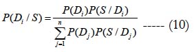
can be obtained from the complete probability formula .jpg) and the obvious relationship P(S)P(Di / S) = P(Di )P(S / Di ). The complete probability formula reflects the postulate that if a system has several possible and incompatible ways to get transferred from the state Dj to the state the probability of such a transfer can be found as the sum of the conditional probabilities of occurrence of each of these ways. The relationship P(S)P(Di / S) = P(Di )P(S / Di). indicates that the probability of the simultaneous occurrence of the symptom and the system condition (diagnosis) Dj can be obtained as the product of these probabilities. As follows from BF,
and the obvious relationship P(S)P(Di / S) = P(Di )P(S / Di ). The complete probability formula reflects the postulate that if a system has several possible and incompatible ways to get transferred from the state Dj to the state the probability of such a transfer can be found as the sum of the conditional probabilities of occurrence of each of these ways. The relationship P(S)P(Di / S) = P(Di )P(S / Di). indicates that the probability of the simultaneous occurrence of the symptom and the system condition (diagnosis) Dj can be obtained as the product of these probabilities. As follows from BF, .jpg)
This is the condition of normalization. The BF (10) is simple, easy to apply and is used therefore in many applied science and engineering problems. Its shortcomings are the large volume of the required input information and strong suppression of infrequent diagnoses. The application of BF in technical diagnostics of electronic and photonic materials and devices enables assessing the reliability of a particular malfunctioning device from the available general information for similar devices manufactured on a massive scale using the same technology. Let us illustrate this statement by a detailed example. It has been established from experience with the given type of devices subjected in actual operation conditions to elevated temperature and random vibrations that 90% of the devices do not typically fail during operation. It has been found also that the diagnostic symptom - an increase in temperature by 20ºC above the normal (specified) level - is encountered in 5% of the devices of interest. The technical diagnostics instrumentation has detected in a particular electron device the following two deviations (“symptoms of failure”) from normal operation conditions: increase in temperature by 20ºC at the heat sink location (symptom S1) and increase in the vibration power spectrum at the device location by (symptom S2). These symptoms might be due to the malfunction of the heat sink (state D1) and/or the malfunction of the vibration protection equipment (state D2). From the previous experience with similar devices and at similar operation conditions it has been established that the symptom S1 (increase in temperature) is not observed at normal operation condition (state D3, and the symptom S2 (increase in the power of the vibration spectrum) is observed in of the cases (devices). It has been established also, based on the accumulated experience with the given type of devices, that of them do not fail during the specified time of operation, of them experience malfunction of the heat sink (state D1), and of the devices experience malfunction of the vibration protection equipment (state D2). Finally, it has been established that the symptom S1 (increase in temperature) is encountered in the state D1 (the malfunction of the heat sink) in of the devices, the state D2 (the malfunction of the vibration protection equipment) - in 40% of the devices; the symptom S2 (increase in the power of the vibration spectrum) is encountered in the state D1 (malfunction of the heat sink) in of the devices, and in state (malfunction of the vibration protection system) - in of the devices. The above information can be summarized in the form of the diagnostics matrix (Table 1).
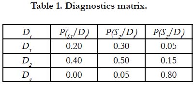

Table 1. Diagnostics matrix.
Thus, this matrix indicates that the symptom S1 (increase in temperature) is encountered in 20% of the cases because of the malfunctioning heat sink (state D1), in 40% of the cases because of the malfunctioning vibration protection system (state D2), and is never observed in normal operation conditions (state D3); the symptom S2 (increase in the power of the vibration spectrum) is encountered in 30% of the cases because of the malfunctioning heat sink (state D1), in 50% of the cases because of the malfunctioning vibration protection system (state D2), and in 5% of the cases in normal operation conditions (state D3), and the symptom S3 (both heat transfer and vibration protection hardware work normally) is encountered in 5% of the cases because of the malfunctioning heat sink (state D1), in 15% of the cases because of the malfunctioning vibration protection system (state D2), and in 80% of the cases in normal operation conditions (state D3).
Let us determine first that the probability that the device, in which the 20ºC increase in temperature has been detected, is still sound. This can be done using the information that 90% of the devices of the type of interest do not typically fail during the designated time of operation and that the symptom S1 (an increase in temperature by 20ºC above the normal level) is encountered in 5% of these devices. The first message tells that the probabilities of the sound condition D1 and the faulty condition D2 in the general population of the devices under operation are P(D1) = 0.9 and P(D2) = 0.1, respectively. The second message tells that the conditional probabilities reflecting the actual situation with the given device are P (S/D1) = 0.05 and P(S/D2) = 0.95: only 5% of the devices function adequately, while 95% of them do not. The question asked is as follows: with this new information about a particular device, how did the expected probability P(D1) = 0.9 that the device of interest is still sound changed? In other words, how could one use the accumulated experience about the operational performance of the large population of this type of devices, considering the results of the actual field information for a particular device? The BF predicts the following probability of the device non-failure (i.e., that device is sound):
.jpg)
Thus, the probability that the device is still sound has decreased dramatically, from for the typical (expected) situation to as low as This happened because of the detected 20ºC increase in temperature and because such an increase is viewed as the device failure. The BF (10) suggests that the factor
.jpg)
could be used to assess, based on the updated reliability information, the change in the initial probability that the device is still sound and if so, its use could be continued with a high level of be much different, if only a slight decrease in the probability of non-failure for the given device, based on the obtained symptom, is detected. Indeed, with P (S/D1) = 0.85 (instead of 0.05) and P(S/D2) 0.15 (instead of 0.95), the factor χ would be as high as χ = 0.9808, would be as high as: P(D1/S) = 0.8827. Let us address now, using the information in Table 1, the performance of the device caused by the possible malfunction of the heat sink and/ or the vibration protection system. The probability
.jpg)
defines the devices state, when both symptoms, S1 (faulty heat sink) and S2 (inadequate vibration protection), have been detected/ observed. This is the probability that the device, for which both symptoms, malfunctioning heat sink and malfunctioning vibration protection system, have been detected, is in the state D1, i.e., failed because of the malfunctioning heat sink. Similarly, one could find the probability P (D2/S1S2) = 0.91 that the device is in the state D2, i.e., failed because of the malfunctioning vibration protection system. Since it is known that the device has failed, it cannot be in the non-failure state D3, and therefore the probability that the device is still sound, despite the detected malfunctions of the heat sink and the vibration protection system, is zero: P(D3/ S1S2) = 0.
Let us determine the probability of the device’s state if the prognostics measurements have indicated that there was no increase in temperature (the symptom S1 did not take place), but the symptom S2 (increase in the power spectrum of the induced vibrations) has been detected. The absence of the symptom S1 means that the symptom - 1 S of the opposite event took place, so that its conditional probability can be of the opposite event took place, so that its conditional probability can be found as 1 1 ( / ) 1 ( / ) i i P S D = − P S D . Changing in the diagnostics matrix in Table 1 the probability P(S1/Di) for the probability 1 ( / )i P S D that the device is found in the state D1, i.e. , that its failure occurred because of the malfunction of the heat sink, we obtain the probability 1 1 2 P(D / S S ) as follows:
.jpg)
Similarly, we obtain:
P(D / S S ) = 0.46 and 3 1 2 P(D / S S ) = 0.41.
Determine now the probabilities of the device states when none of the two symptoms took place. By analogy we obtain:
.jpg)
Similarly, we have:
P(D / S S ) = 0.05; 3 1 2 P(D / S S ) = 0.92. Thus, when both symptoms, S1 adn S2, are observed, the state D1 (failure occurred because the heat sink is malfunctioning) has the probability of occurrence of 0.91. When none of these symptoms are observed, the normal state, D3, takes place and is characterized by the probability 0.92. Hence, the normal state D3 is somewhat more likely to occur than the state, when both symptoms, S1 and S2, are observed. When the symptom S1 the states S2 (vibration protection system is not working properly) and S3 (both heat transfer and vibration protection hardware work normally) are and respectively.
One could either accept this information and act accordingly, i.e., go ahead with a conclusion that it is the elevated temperature and not the elevated vibration that should be taken care of, or, since these probabilities are rather close, one might decide on seeking additional information. Such information could be based on generated additional observations. Alternatively, one could use other sources to obtain more accurate and more convincing diagnostics information (such as, e.g., modeling or additional measurements). Thus, the first step of the TSC enables one to identify, on the probabilistic basis, the malfunctioning device(s) and the most likely cause(s) that have resulted in the device failure. The objective of the next step is to assess, using BAZ equation, the remaining useful lifetime (RUL) of the detected the malfunctioning device(s).
Step 2. Application of BAZ equation to predict the RUL of an EP product
Assume that FOAT has been conducted at the design stage with an objective to determine the process parameters anticipated by the BAZ model, and that the first stage tests have been carried out at two temperature levels, T1 and T2, with the temperature ratio of T1/T2 = 0.95 and the recorded time-to-failure ratio t1/t2 = 1.5. Testing was terminated when half of the population failed: Q1 = Q2 = 0.5. Then the equation
.jpg) can be obtained for the sought dimensionless time τ1 = τ0/t1. This equation has the following solution:
can be obtained for the sought dimensionless time τ1 = τ0/t1. This equation has the following solution: .jpg)
that has been obtained by the trial-and-error (interpolation) technique. If Newton’s method for solving transcendental equations is used, then, by putting, e.g., τ0 = 10-4 as the initial (zero) approximation and using Newton’s recurrent formula to compute higher approximations, the following τ values could be obtained: τ1 = 2.73194x10⁻⁴; τ2 = 4.06515x10⁻⁴; τ3 = 4.32841x10⁻⁴; τ4 = 4.33475x10⁻⁴. The latter result agrees well with the result obtained using trial-and-error technique.
Let FOAT be conducted at the temperature of T = 450° K at two stress levels with the stress ratio of, say, σ1/σ2 = 1.2. Testing is run until half of the population failed (Q1 = Q2= 0.5), and the recorded time ratio, when failures occurred, was t1/t2 = 1.5. In this example it is assumed that the time constant τ0 in the BAZ equation is known from the previous FOAT. With this constant known, we calculate the τ0/t1 ratio for the new time t1. If this ratio of the time constant t1 to the testing time t1 is, say, τ0/t1 = 4.0x10⁻⁴, then the loading/stressing σ1 related energy γσ1 can be evaluated as follows:
.jpg)
The ratio of the two energies (mechanical and thermal) is therefore
.jpg)
This ratio is larger for larger loadings and lower temperatures. The ratio of the stress-free activation energy to the thermal energy is
.jpg)
The effective activation energy, when the loading/stress σ1 is applied, is as follows: 0 1 U =U −γσ = 0.3962 − 0.0786 = 0.3176eV.
When the stress σ2 is applied, this energy is
.jpg)
Let us assume that the FOAT-based and BAZ-based calculations carried out at the operation temperature of T = 90ºC = 363K T = 90ºC = 363K have indicated that the time factor is τ0 = 10-4 sec; the ratio of the stress-free activation energy to the temperaturerelated energy is U0/kT = 30.0; and the ratio of the stress-related energy to the thermal energy is γσ/kT = 1.0. Then the BAZ formula (1) results in the following projected lifetime:
.jpg)
days in the case of the 20ºC increase in temperature. Thus, the increase in temperature should be, considering the information obtained in this example, of greater concern than the increase in the vibration response (the output vibration spectrum). Also, based on the BF prediction, the malfunction of the device due to the increased temperature is more likely than because of the faulty vibration protection system.
We conclude that the output of this, second, TSC stage is the quantified, on the probabilistic basis, RUL of the device(s) of interest. As has been indicated, if the assessed RUL time is still long enough, no action might be needed, if not -corrective restoration action becomes necessary. In any event, after the first two TSC steps have been carried out, the devices are put back into operation, provided that the assessed probability of their continuing failure-free operation is found to be satisfactory. If failure nonetheless occurs, the third step should be undertaken to update the predicted reliability. Statistical BD, in which the probability of failure is treated as a random variable, is suggested to be used at this third step.
Step 3. Application of BD to update reliability information, when failures still occur
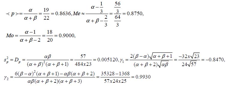
Let the performance of five “suspicious” (malfunctioning) devices is monitored, and one of them failed. Let us determine the BD characteristics for four successes and one failure (α = 4,β =1) . We have: α =α +1 = 5,β = β +1 = 2, and the distribution characteristics are:
.jpg)
With α β (there are more successes than failures), the distribution skews to the higher probabilities of non-failure, and the mode (the maximum value, of the probability density function) is higher than the mean value and the median. Let no failures have been observed after the first two TSC steps have been carried out. Let us determine the expected number of successes (non-failures) as a function of the probability of non-failure. Assuming zero failures (β = 0,β =1) we have: 2 1 1 p p α − = − If the mean value of the probability of non-failure is p = 0.7143, then α =1.5002. Since α value has to be expressed by an integer, one should assume either α =1(α = 2) or α = 2(α = 3) . Then
.jpg)
when α = 3,β =1. In both cases, it is a triangular distribution: the mode remains the same, and is at P =1. The mean and the median increase in the caseα = 3,β =1. in comparison with the case α = 2,β =1, because of a larger number of successes. The variance reduces, because of the improved information, and the skewness (shift in the direction of higher probabilities of non-failure) and the kurtosis (“peakedness”) of the distribution increase.
Assume now that the predicted (anticipated) probability of nonfailure is as high as p = 0.95. Despite such a high probability of non-failure, the product exhibited nonetheless a field failure. Let us determine, based on this additional information, the revised (updated) estimate of the actual operational probability of non-failure. Assuming that the anticipated (projected) number of failures was zero (β = 0,β =1) prior to putting the device(s) into operation, and using the formula for the number α of anticipated non-failures from the previous example, we obtain, with
.jpg)
For a new posterior failure, with α =18(α =19) and β =1(β = 2),the revised characteristics of the BD for the probability of non-failure are
.jpg)
Thus, because of the occurrence of the unexpected failure, the actual probability of non-failure of the product is only 90.45%, and not 95%. Note that this result, obtained assuming a 95% nonfailure level, indicates that after the first failure has occurred, as many as nineteen additional continuous non-failures (successes), i.e., 18+19 = 37 successes and one failure, would have to be recorded (observed) in order to return the device’s dependability (probability of non-failure) to its original specified estimate of 95%.
We addressed above a situation where one failure has occurred. Let us examine a situation with two failures. In this case one should put α =18(α =19) and β = 2(β = 3) and the characteristics of the BD for the probability of non-failure become as follows:
Thus, the employed technique for updating the operational probability of non-failure indicates that this probability was reduced by about 9.12%, compared to the projected probability of 95%, and by an additional 4.52% with respect to the situation with a single failure. The mean, the median and the mode of the distribution have also decreased, and because of the higher number of failures, the variance has increased, and the skewness and the kurtosis have decreased. The application of the BD is therefore a useful and an effective means for updating reliability information.
We conclude that the application of the suggested TSC methodology enables improving the state of the art in the field of the electronic products reliability prediction and assurance.
Predicted Static Fatigue Lifetime of an Optical Silica Fiber
BAZ equation can be effectively employed as an attractive replacement of the widely used today purely empirical power law relationship for assessing the static fatigue (delayed fracture) lifetime of optical silica fibers. In the analysis below the combined action of tensile loading and an elevated temperature is addressed.
Let, e.g., the following input FOAT information is obtained at the FOAT first step for a polyimide coated fiber intended for elevated temperature operations: 1) After 1 t =10h of testing at the temperature of T1 = 300 C = 573 K , under the stress of σ = 420kg / mm2 , 10% of the tested specimens failed, so that the probability of non-failure is 1 P = 0.9; 2) After of testing at the temperature of 0 0 2 T = 350 C = 623 K under the same stress, 25% of the tested samples failed, so that the probability of non-failure is 2 P = 0.75. Forming the equation (10) and introducing notations
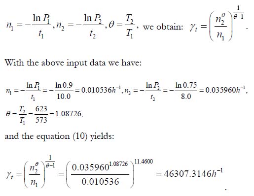
At the second step FOAT has been conducted at the stresses of σ1 = 420kg / mm and 2 2 σ = 320kg / mm at T = 3500C = 6230K, and it has been confirmed that 10% of the tested samples under the stress of 2 1 σ = 420kg / mm failed after 1 t =10.0h of testing, so that P1 = 0.9. The percentage of failed samples tested at the stress
of 2 2 σ = 320kg / mm was 5% after 2 t = 24h of testing, so that 2 P = 0.95. Then, according to the developed methodology, the ratio of the stress sensitivity factor to the thermal energy is: 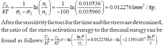
If, e.g., the stress 2 1 σ =σ = 320kg / mm is applied for t = 24h and the acceptable probability of non-failure at the end of this time is, say, P = 0.99, then the ratio of the zero stress activation energy to the thermal energy is
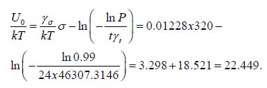
This result indicates that the activation energy U0 is determined primarily by the property of the silica material (second term), but is affected also, to a lesser extent, by the level of the applied stress.
The fatigue lifetime can be determined for the acceptable (specified) probability of non-failure as 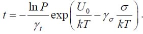
This formula indicates that if the probability of non-failure is low, the expected lifetime could be quite long. If, e.g., the applied temperature is T = 3250C = 598K, the applied tensile stress is 5.0kg/mm2, and the acceptable probability of non-failure is only P = 0.8, then
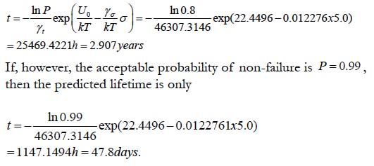
Thus, the 23.75% increase in the accepted probability of nonfailure resulted in the 22.2 fold decrease in the lifetime.
Predicted Low-Cycle Fatigue Life-Time Of Solder
Joint Interconnections
While low-cost and short time-to-market that are the main driving forces in commercial electronics, it is high operational reliability that is of the predominant importance in aerospace, military, medical, long-haul communication and other areas of electronic and photonic engineering, in which highly reliable performance is required. Such performance cannot be achieved, if the underlying physics of the possible failure(s) is not well understood and the never-zero probability of failure of the product of interest is not addressed. Highly focused and highly cost effective reliability physics based FOAT, an essential part of the PDfR concept geared to a flexible, easy-to-use and physically meaningful constitutive BAZ equation should be conducted whenever appropriate and possible. In the analysis that follows it is shown how this could be done for an electronic device subjected during FOAT to temperature cycling.
Using BAZ model, the probability of non-failure of a vulnerable material, such as, e.g., solder joint interconnection experiencing inelastic strains during temperature cycling can be sought in the form:
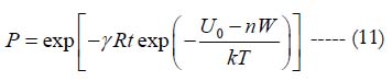
Here U0 is the activation energy and is the characteristic of the solder material’s propensity to fracture, W is the damage caused by a single temperature cycle and measured, in accordance with Hall’s concept, by the hysteresis loop area of a single temperature cycle for the strain of interest, T, K is the absolute temperature (say, the cycle’s mean temperature), n is the number of cycles, k = 8.6173x10⁻⁵eV /0 K is Boltzmann’s constant, t, sec, is time, R, Ω, is the measured (monitored) electrical resistance at the peripheral joint location, and γ is the sensitivity factor for the resistance.
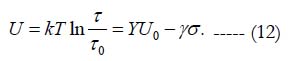
The above equation makes physical sense. Indeed, the probability P of non-failure is zero at the initial moment of time t = 0 of non-failure is zero at the initial moment of time R of the joint material is zero; this probability decreases, because of material aging and structural degradation with time, and not necessarily only because of temperature cycling; it is lower for higher electrical resistance (a resistance as high as, say, 450Ω, can be viewed as an indication of an irreversible mechanical failure of the joint); materials with higher activation energy U0 have a lower probability of possible failure; the increase in the number of cycles n leads to lower effective activation energy 0 U =U − nW , and so does the level of the energy W of a single cycle. There is an underlying entropy related consideration for the equation (12). It could be shown that the maximum entropy of the distribution (1) takes place at the MTTF τ expressed as 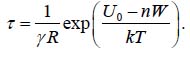
Mechanical failure, associated with temperature cycling, takes place, when the number of cycles n is 
When this condition takes place, the temperature in the denominator in the parentheses of the above equation becomes irrelevant and yields: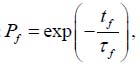
where Pf is the measured probability of non-failure for the situation when failure occurred because of temperature cycling, and 
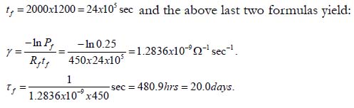
is the MTTF. If, e.g., 20 devices have been temperature cycled and the high resistance Rf = 450Ω, considered as an indication of failure was detected in 15 of them, then 0.25 f P = . If the number of cycles during such FOAT was, say, nf = 2000, and each cycle lasted, say, for 20min=1200sec., then the time at failure is 2000 1200 24 105 sec ft = x = x and the above last two formulas yield:
According to Hall’s concept, the energy W of a single cycle should be evaluated, by running a specially designed test, in which strain gages should be used. Let, e.g., in the above tests this energy (the area of the hysteresis loop) was W = 2.5x10⁻⁴ eV. Then the stress-free activation energy of the solder material is 4 0 2000 4.5 10 0.9 . f U = n W = x x − = eV In order to assess the number of cycles to failure in actual operation conditions one could assume that the temperature range in these conditions is, say, half the accelerated test range, and that the area of the hysteresis loop is proportional to the temperature range. Then the number of cycles to failure is
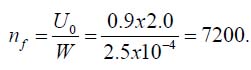
If the duration of one cycle in actual operation conditions is one day, then the time to failure will be tf = 7200days = 19.726years.
It is noteworthy that FOAT could be viewed as an extension of the HALT and could be conducted within the framework of HALT. For new products, when there is no experience accumulated yet and best practices do not yet exist, FOAT can be conducted even instead of HALT, or as the first step to an adequate HALT. Future work should include, first of all, actual FOAT and information on actual operational lifetimes.
Predicted Long-Term Reliability of IC Devices
From Yield Information
Modified BAZ constitutive model is applied to predict the reliability of integrated circuits. The model accounts for the impact of physical defects and process variations on the stress-free activation energy, which is viewed as a critical material's property. It is shown that the probability of non-failure (reliability) and the corresponding MTTF can be evaluated from the FOAT geared to the modified BAZ model. The BAZ model is further modified for this application. It is considered that the stress-free energy U0 is affected by physical defects and process variations that reduce this energy and, hence, the IC yield (0 ≤ Y ≤ 1). Then, the expression for the effective activation energy is assumed as
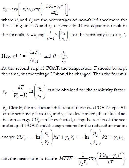
If the applied voltage V is considered as a physically meaningful stressor, then the equation (5) for the probability of non-failure can be presented in the form
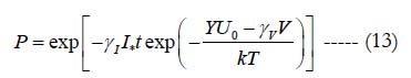
The equation makes physical sense. Indeed, the probability of non-failure decreases with time, temperature, leakage current, and the applied voltage and is higher for larger stress-free activation energy. The equation (13) contains three unknowns: the sensitivity factors γ1 and γV, and the activation energy U0. These unknowns could be found from the FOAT. Testing should be conducted in two steps. At the first step, testing should be carried out for two temperature levels, T1 and T2, while keeping the effective energy 0 V YU −γ V in the numerator of the above formula unchanged. Then the test data result in two equations
Six critical processes typically responsible for the yield loss in the semiconductor technology practice are considered: P+ diffusion, N+ diffusion, silicon-dioxide formation, contact formation, via formation, and metal layer formation. In-line yield measurements made on the corresponding test structures are presented in Table 2. Let leakage current of I* = 0.5 μA is viewed as a definition of failure. Having in mind that the proposed model uses two stressors (temperature and voltage), we selected two temperature and two voltage values to be applied (stressing the test structures) in two consecutive FOAT steps. The first step of testing was conducted at temperatures T1 = 25°C = 298 K and T2 = 50°C = 323 K, until half of the test specimens failed, so that P1= 0.5 and P2 = 0.5. Then the θ ratio can be calculated as: θ = T1/T2 = 323/298 = 1.0839.
The times necessary for the failure of a half of the measured test structures (a hundred samples) and the corresponding temperature sensitivity factor are presented in Table 3.
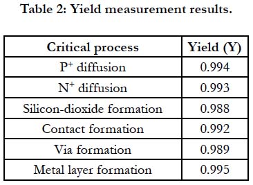
Table 2: Yield measurement results.
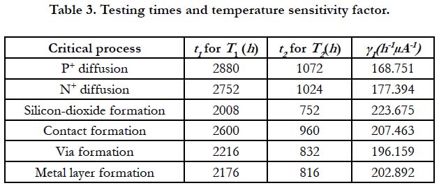
Table 3. Testing times and temperature sensitivity factor.
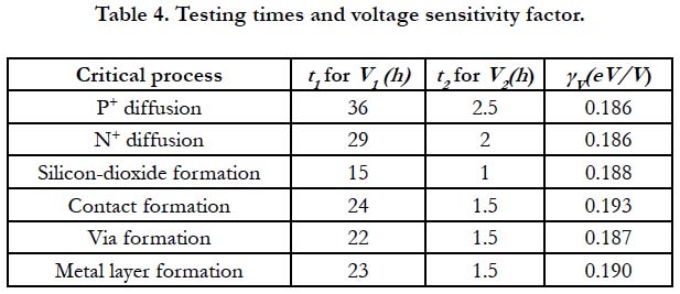
Table 4. Testing times and voltage sensitivity factor.
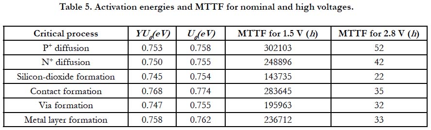
Table 5. Activation energies and MTTF for nominal and high voltages.
At the second step, testing was conducted at a temperature of T = 50°C = 323° K, first at a voltage V1 = 2.8 V first at a voltage V2 = 3.2 V. Testing was conducted until a half of the measured test structures (a hundred samples) failed (P1 = P2 = 0.5). The times necessary for the failure of a half of the measured test structures and the corresponding voltage sensitivity factor are presented in Table 4. Then the formula (13) can be used to calculate the reduced and defect-free failure activation energies. These results based on the measured data can be used for reliability predictions. The activation energies and the MTTF for two voltage values are shown in Table 5. Thus, a modified multi-parametric BAZ model that establishes the link between the yield and reliability (probability of non-failure) has been suggested. The proposed modification of the model takes into account the reduction of the stress-free failure activation energy caused by physical defects and process variations defining the yield as a correction parameter. The presented application example shows the first promising results. The next step will be to compare the model predictions with reliability test data from the field.
Use of BAZ equation to quantify BIT effort
BIT [26-29] is an accepted practice for detecting and eliminating early failures in newly fabricated electronic products prior to shipping the “healthy” ones that survived BIT to the customer(s). BIT can be based on temperature cycling, elevated temperatures, voltage, current, humidity, random vibrations, etc., and/or, since the principle of superposition does not work in reliability engineering, - on the appropriate combination of these stressors. BIT is a costly undertaking: early failures are avoided and the infant mortality portion of the bathtub curve (BTC) is supposedly eliminated at the expense of the reduced yield. But what is even worse, is that the elevated BIT stressors (temperature cycling, elevated temperatures, voltage, current, humidity, random vibrations, etc., or their appropriate combination) might not only eliminate “freaks,” but could cause permanent damage to the main population of the “healthy” products. BIT should be therefore well understood, thoroughly planned and carefully executed. It is unclear, however, whether BIT is always needed, nor to what extent the current practices are adequate and effective. HALT that is currently employed as a BIT vehicle is a “black box” that tries “to kill many birds with one stone” and is unable to provide any trustworthy information on what it actually does. It remains unclear what is actually happening during, and as a result of, the HALT-based BIT and how to effectively eliminate “freaks,” while minimizing the testing time, reducing its cost and avoiding damaging the sound devices. When HALT is relied upon to do the BIT job, it is not even easy to determine whether there exists a decreasing failure rate with time. There is, therefore, an obvious incentive to develop ways, in which the BIT process could be better understood, trustworthily quantified, effectively monitored and possibly optimized. Accordingly, in this analysis some important BIT aspects are addressed for a packaged EP product comprised of numerous mass-produced components. We intend to shed some quantitative light on the BIT process, and, since nothing is perfect (the difference between a highly reliable process or a product and an insufficiently reliable one is merely in the levels of their never-zero probability of failure), such a quantification should be done on the probabilistic basis. Particularly, a suitable criterion is intended to be developed to answer the fundamental “to burn-in or not to burn-in” question, and if BIT is decided upon, - to find a way to quantify its outcome. This could be done using BAZ model.
We address the role and significance of the following important factors that affect the testing time and the stress level: the random statistical failure rate (SFR) of mass-produced components that the product of interest is comprised of; the way to assess, from the highly focused and highly cost-effective FOAT, the activation energy of the “freak” population; the role of the applied stressor(s); and, most importantly, the probabilities of the “freak” failures depending on the duration of the BIT effort, and a way to assess, using BAZ equation, these probabilities as functions of the duration and level of the BIT, and the variance of the random SFR of the mass-produced components that the product of interest is comprised of. It is shown that the BTC based timederivative of the failure rate at the BTC initial moment of time can be considered as a suitable criterion of whether BIT for a packaged IC device should be, or does not have to be conducted. It is shown also that this criterion is, in effect, the variance of the random SFR of the mass produced components that the manufacturer of the given product received from numerous vendors, whose commitments to reliability were unknown, and therefore the random SFR of these components might vary significantly, from zero to infinity. Based on the general formula for the nonrandom SFR of a product comprised of such components, the solution for the case of normally distributed random SFR of the constituent components has been obtained. This information enables answering the “to burn-in or not to burn-in” question in electronics manufacturing.
If BIT is decided upon, the BAZ model can be employed for the assessment of its required duration and level. This model has been recently generalized in application to microelectronics reliability and used as an effective constitutive equation in the PDfR approach for packaged IC devices, when there is an intent and need to evaluate the probability of failure and the corresponding lifetime of a packaged IC product.
It is shown that the bathtub-curve (BTC) based time-derivative of the failure rate at the BTC initial moment of time can be considered as a suitable criterion of whether BIT for a packaged IC device should or does not have to be conducted. It is shown also that this criterion is, in effect, the variance of the random SFR of the mass-produced components that the manufacturer of the product of interest received from numerous vendors, whose commitments to reliability were unknown, and therefore the random SFR of these components might very well vary significantly, from zero to infinity. Based on the general formula for the nonrandom SFR of a product comprised of such components, the solution for the case of normally distributed random SFR of the constituent components was obtained. This information enables answering the “to burn-in or not to burn-in” question in electronics manufacturing.
If BIT is decided upon, BAZ model can be employed for the assessment of its required duration and level. Our analyses shed light on the role and significance of important factors that affect the testing time and stress level: the random SFR of massproduced components that the product of interest is comprised of; the way to assess, from the highly focused and highly cost effective FOAT, the activation energy of the “freak” population; the role of the applied stressor(s); and, most importantly, - the probabilities of the “freak” failures depending on the duration of the BIT effort. These factors should be considered when there is an intent to quantify and, eventually, to optimize the BIT’s procedure.
This fundamental question is addressed using two mutually complementary and independent analyses:
1) the analysis of the configuration of the infant mortality portion (IMP) of a BTC obtained for a more or less well established manufacturing technology of interest; and 2) the analysis of the role of the random SFR of the mass-produced components that the product of interest is comprised of, as far as the effect of this SFR on the nonrandom initial SFR of the product is concerned. The desirable steady-state portion of the BTC commences at the BIT’s end as a result of the interaction of two major irreversible time-dependent processes: the “favorable” statistical process that results in a decreasing failure rate with time, and the “unfavorable” physics-of-failure-related process resulting in an increasing failure rate. The first process dominates at the IMP of the BTC and is considered here. The IMP of a typical BTC, the “reliability passport” of a mass-produced electronic product, can be approximated as:
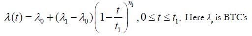
Here λo is BTC’s steady-state minimum, λ1 is its initial (highest) value at the beginning of the IMP, t1 is the duration of the IMP, the exponent n1 is n1 = β1 / 1-β1, and β1 is the fullnesses of the BTC’s IMP.
This fullness is defined as the ratio of the area below the BTC to the area 1 0 1 (λ −λ )t of the corresponding rectangular. The exponent n1 changes from zero to one, when the fullness β1 changes from zero to 0.5. The time derivative of the failure rate at the initial moment of time 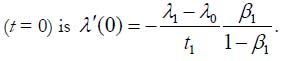
If this derivative is zero or next-to-zero, this means that the IMP of the BTC is parallel to the time axis (so that there is, in effect, no IMP at all), that no BIT is needed to eliminate this portion, and “not to burn-in” is the answer to our basic question: the initial value λ1 of the BTC is not different from its steady-state λ0 value. What is less obvious is that the same result takes place for β1/t1=0.
This means that although the BIT is needed, the testing could be short and low level, because there are not too many “freaks” in the manufactured population and because, although these “freaks” exist, they are characterized by very low probabilities of non-failure, so that the planned BIT process could be a next-toan- instantaneous one. The maximum value of the fullness β1 is β1 = 0.5. This corresponds to the case when the IMP of the BTC is a straight line connecting the initial, λ1, and the steady-state, λ0, BTC values. The derivative 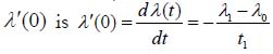
in this case, and this seems to be the case, when the BIT is mostly needed. The non-random time dependent SFR
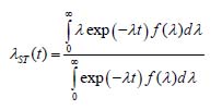
can be obtained from the probability density distribution function f(t) for the random SFR λ. When this failure rate is normally distributed, i.e., when its probability density function is
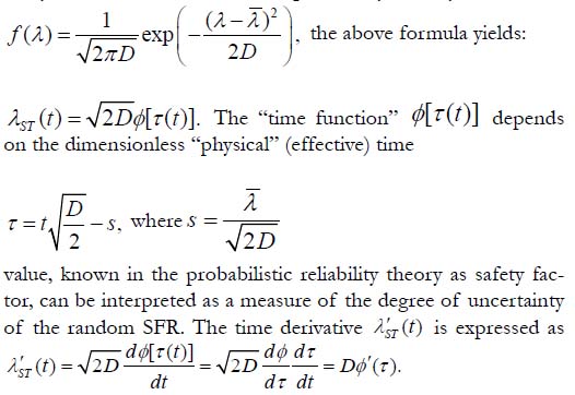
It can be shown that the derivative φ ′(τ ) at the initial moment of time (t = 0) is equal to −1.0, so that
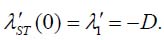 This result explains the physical meaning of this derivative: it is the variance (with a “minus” sign, of course) of the random SFR of the constituent components.
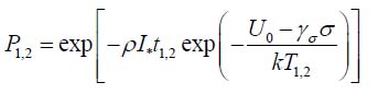
The BAZ model suggests a simple, easy-to-use, highly flexible and physically meaningful way to evaluate of the probability of failure of a material or a device after the given time in testing or operation at the given temperature and under the given stress or stressors. Using this model, the probability of non-failure during the BIT can be sought as 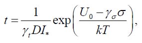
Here is the variance of the random SFR of the mass-produced components, I is the measured/monitored signal (such as, e.g., leakage current, whose agreed-upon high value I* is considered as an indication of failure; or an elevated electrical resistance, particularly suitable for solder joint interconnections), t is time, σ is the “external” stressor, U0 is the activation energy (unlike in the original BAZ model, this energy may or may not be affected by the level of the external stressor), T is the absolute temperature, γσ is the stress sensitivity factor and γt is the time/variance sensitivity factor. The above distribution makes physical sense. Indeed, the probability P decreases with an increase in the variance D, in the time t, in the time I* of the leakage current at failure and in the temperature T, and increases with an increase in the activation energy U0.
As has been shown above, the maxima of the entropy and the probability of non-failure take place at the moment of time
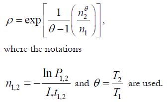
accepted as the MTTF. There are three unknowns in this expressions: the product ; tρ =γ D the stress-sensitivity factor γσ and the activation energy U0. These unknowns could be determined from a two-step FOAT. At the first step testing should be carried out for two temperatures, T1 and T2, but for the same effective activation energy U = U0 - γσσ Then the relationships
for the measured probabilities of non-failure can be obtained. Here t1,2 are the corresponding times and I* is the leakage current at failure. Since the numerator 0 U =U −γσ in these relationships is kept the same, the amount tρ =γ D can be found as
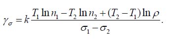
The second step of testing is aimed at the evaluation of the stress sensitivity factor γσ and should be conducted at two stress levels σ1 and σ2 (say, temperatures or voltages). If the stresses σ1 and σ2 are thermal stresses determined for the temperatures T1 and T2, they could be evaluated using a suitable stress model. Then
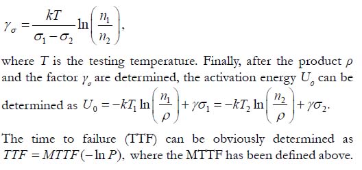
If, however, the external stress is not a thermal stress, then the temperatures at the second step tests should preferably be kept the same. Then the ρ value will not affect the factor γσ, which could be found as
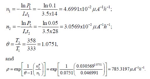
Let, e.g., the following data were obtained at the first step of FOAT: 1) After t1 = 14h of testing at the temperature of T1 = 60°C = 333°K, 90% of the tested devices reached the critical level of the leakage current of I* = 3.5μA and, hence, failed, so that the recorded probability of non-failure is P1 = 0.1; the applied stress is elevated voltage σ1 = 380V; 2) After t2 = 28h of testing at the temperature of T2 = 85°C = 358°K, 95% of the samples failed, so that the recorded probability of non-failure is P2 = 0.05. The applied external stress is still elevated voltage of the level σ1 = 380V. Then
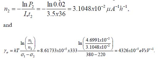
At the second step of FOAT one can use, without conducting additional testing, the above information from the first step, its duration and outcome, and let the second step of testing has shown that after t2 = 36h of testing at the same temperature of T1 = 60°C = 333°K, 98% of the tested samples failed, so that the predicted probability of non-failure is P2 = 0.02. If the stress σ2 is the elevated voltage σ2 = 220V, then
The zero-stress activation energies calculated for the parameters and n1 and n2 the stresses σ1 and σ2 should be and are the same:
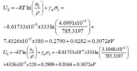
(to make sure that there was no calculation error). No wonder that these values are considerably lower than the activation energies of “healthy” products. Many manufacturers consider as a sort of “rule of thumb” that the level of 0.7eV can be used as an appropriate tentative number for the activation energy of healthy electronic products. In this connection it should be indicated that when the BIT process is monitored and the activation energy U0 is being continuously calculated based on the number of the failed devices, the BIT process should be terminated, when the calculations, based on the FOAT data, indicate that the energy U0 starts to increase. The calculated data show also that this energy slightly increases with an increase in the level of loading. This increase is, however, only about 5-8%. The MTTF is
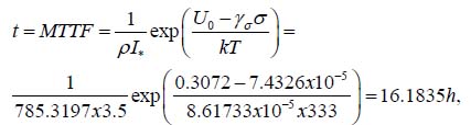
and the TTF values calculated as TTF = MTTFx(ln P) are shown in Table 6.
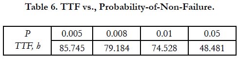
Table 6. TTF vs., Probability-of-Non-Failure.
Clearly, the probabilities of non-failure for successful BITs should be low enough. It is clear also that the BIT process should be terminated when the calculated probabilities of non-failure and the activation energy U0 start rapidly increasing. Although our BIT analyses do not suggest any straightforward and complete way of how to optimize BIT, they nonetheless shed useful and insightful light on the significance of some important factors that affect the BIT’s need, and, if decided upon, - its required time and stress level for a packaged product comprised of mass-produced components.
Conclusion
Application of BAZ equation in EP RP problems, and particularly in those encountered in aerospace engineering, enables quantifying, on the probabilistic basis, the performance (actually, the probability of failure under the anticipated loading conditions and after the given operation time) and the lifetime of an electronic or a photonic material. This makes a viable device into a reliable product, with the predicted, adequate and, when necessary and appropriate, even specified never-zero probability of failure in the field.
References
- SN Zhurkov. The Problem of the Strength of Solids. Bulletin of the USSR Academy of Sciences. 1957(11):78-82.
- Zhurkov AN. Kinetic concept of the strength of solids. Int J Fract Mech. 1965;1:311-23.
- Arrhenius S. About the heat of dissociation and the influence of temperature on the degree of dissociation of the electrolytes. Journal of physical chemistry. 1889 Jul 1;4(1):96-116.
- Boltzmann L.Studies on the balance of living power. Scientific papers. 1868;1:49-96.
- Boltzmann L. The second law of thermodynamics. Populare Schriften, Essay 3, address to a formal meeting of the Imperial Academy of Science, 29 May 1886, reprinted in Ludwig Boltzmann. Theoretical physics and philosophical problem, SG Brush (Trans.). Boston: Reidel.(Original work published 1886). 1974.
- Suhir E, Kang SM. Boltzmann–Arrhenius–Zhurkov (BAZ) model in physics-of-materials problems. Modern Physics Letters B. 2013 May 30;27(13):1330009.
- Suhir E, Rafanelli AJ. Applied probability for engineers and scientists. McGraw-Hill. 1992.
- Suhir E. Accelerated life testing (ALT) in microelectronics and photonics: its role, attributes, challenges, pitfalls, and interaction with qualification tests. J Electron. Packag.. 2002 Sep 1;124(3):281-91.
- E. Suhir. Probabilistic Design for Reliability. Chip Scale Reviews.2010;14(6).
- Suhir E. When reliability is imperative, ability to quantify it is a must. IMAPS Advanced Microelectronics. 2012 Jul.
- Suhir E.Could electronics reliability be predicted, quantified and assured?. Microelectronics Reliability. 2013 Jul 1;53(7):925-36.
- Suhir E. Electronics reliability cannot be assured, if it is not quantified. ChipScale Reviews. 2014 Mar.
- Suhir E, Yi S. Probabilistic design for reliability (PDfR) of medical electronic devices (MEDs): when reliability is imperative, ability to quantify it is a must. Journal of SMT. 2017;30(1).
- E. Suhir, “Failure-Oriented-Accelerated-Testing (FOAT) and Its Role in Making a Viable IC Package into a Reliable Product”, Circuits Assembly, 2013.
- Suhir E. The Role of Failure-Oriented-Accelerated-Testing for Field Functional IC Packages. 2013.
- Suhir E. HALT, FOAT and their role in making a viable device into a reliable product. In 2014 IEEE Aerospace Conference. 2014 Mar 1; 1-9.
- Suhir E. What could and should be done differently: failure-oriented-accelerated- testing (FOAT) and its role in making an aerospace electronics device into a product. Journal of Materials Science: Materials in Electronics. 2018 Feb 1;29(4):2939-48.
- Suhir E. Three-step concept in modeling reliability: Boltzmann–Arrhenius– Zhurkov physics-of-failure-based equation sandwiched between two statistical models. Microelectron. Reliab. 2014 Oct;54:2594-603.
- Suhir E, Bechou L, Bensoussan A. Technical Diagnostics in Electronics: Application of Bayes Formula and Boltzmann-Arrhenius-Zhurkov (BAZ) Model. 2012.
- Setchell RE. Reduction in fiber damage thresholds due to static fatigue. In Laser-Induced Damage in Optical Materials. International Society for Optics and Photonics.1994 1995 Jul 14; 2428:.54-65.
- Suhir E. Static fatigue lifetime of optical fibers assessed using Boltzmann–Arrhenius– Zhurkov (BAZ) model. Journal of Materials Science: Materials in Electronics. 2017 Aug 1;28(16):11689-94.
- Hall P. Forces, moments, and displacements during thermal chamber cycling of leadless ceramic chip carriers soldered to printed boards. IEEE Transactions on Components, Hybrids, and Manufacturing Technology. 1984 Dec;7(4):314-27.
- E. Suhir. Making a Viable Medical Electron Device Package into a Reliable Product. Advancing Microelectronics, Medical Electronics, IMAPS.2019;46(2).
- Suhir E, Stamenkovic Z. Using yield to predict long-term reliability of integrated circuits: Application of Boltzmann-Arrhenius-Zhurkov model. Solid-State Electronics. 2020 Feb 1;164:107746.
- Suhir E. Low-Cycle-Fatigue Failures of Solder Material in Electronics Packaging: Analytical Modeling Enables to Predict and Possibly Prevent Them-Review. Journal of Aerospace Engineering and Mechanics. 2018 Apr 2;2(1).
- Kececioglu D. Burn-in testing: its quantification and optimization. Prentice Hall; 1997.
- Burn-In. MIL-STD-883F: Test Method Standard, Microchips. Method 1015.9; US DoD: Washington, DC, USA; 2004.
- Suhir E. To Burn-In, or Not to Burn-In: That’s the Question. Aerospace. 2019 Mar;6(3):29.
- E.Suhir. “Burn-in Testing (BIT): Is It Always Needed?”. IEEE ECTC, Orlando, Fl; 2020.
- Suhir E. Analytical stress-strain modeling in photonics engineering: its role, attributes and interaction with the finite-element method. Laser Focus World. 2002 May;14:611-5.
- E. Suhir. Analytical Thermal Stress Modeling in Electronic and Photonic Systems. ASME Applied Mech. Reviews. 2009: 62(4).
- Suhir E. Analytical modeling enables explanation of paradoxical behaviors of electronic and optical materials and assemblies. Advances in materials Research. 2017 Jun 1;6(2):185.
- E.Suhir. Application of Analytical Modeling in the Design for Reliability of Electronic Packages and Systems. Springer Encyclopedia of Continuum Mechanics; 2019.